Deformable Attention - multiple input views
How would attention mechanism work in transformers when the space of the multiple inputs live in separate dimensions
Deformable attention is very efficient in regards to reducing the computation of regular attention. Where every tensor is attending to one another. Meaning our computation scales quadratically with the amount of input vectors into the transformer. This is something deformable attention combats by allowing the vectors to sample locations of interest.
Regular attention:
This equation shows how every token in our Query matrix communicates with every token in our Key matrix. Deformable acts differently, it comes with learned sampling points per query:
M is our M attention heads, while K is our sampling points per attention head.
- : content of our query tokens
- : reference points of our queries
- : input feature map: which we will be sampling from.
- : output projection.
- : is the attention weight for the k'th sampling location. Where =1
- : value projection for head M
- : sampling location offsets for the query.
- : sums the k weighted samping tokens for that head.
Breaking it down: doesn't actually multiply with the sampling location, instead its a lookup reference. The actual feature exctraction happens via billinear interpolation, but that's outside of this blogs scope. Now we take this feature and multiply it with out value projection for head M: , resulting in a vector. Once we have extracted the value, we then multiply it with our attention scalar . In the original paper it's written capitalized, but as it's a scalar I will follow the conventions and write it lowercase. We then sum the values of all the sampled feature vectors, then multiply it by our matrix, which results in a vector. Which will then be our new query vector value.
Now let's say we are using this architecture within the context of detecting birds. This is typically a very straightforward problem to solve. As typically the contrast between the bird and the background sky is very apparent. However what happens when brids cluster into flocks.
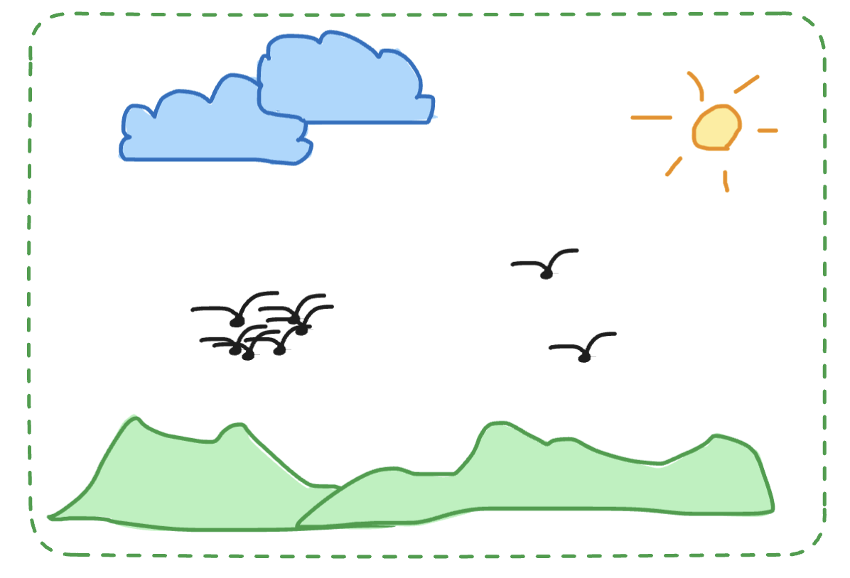
As soon as the birds start clustering together the detection problem starts becoming more complex. If we are working with the DETR architecture, a go-to solution would be to select an ealier level from the backbone and send that into our transformer.
This then increases compute significantly (if this were regular DETR then it would increase quadratically). There are also other techniques, such as moving towards h-detr, dino-detr, co-detr, etc. that will help refine the accuracy further. But besides that, let's say you have a separate view of these birds, focused on the cluster, with higher focus/resolution.
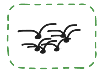
Now this focused frame has a more dense bird representation, and will have an easier time distinguishing birds from one another.
Now let's visualize the actual DETR architecture. It can be broken down to 3 main components:
- Backbone
- Encoder
- Decoder
Our image will be parsed through our backbone, extracting its features. These feature tokens are then flattened and sent into our encoder. This will be self attention across the encoders, where in the case of Deformable attention, we will by defualt be sampling 4 locations per feature token. We will then perform this operation x times depending on how many encoder layers you have selected. Now the feature tokens has spoken with each other, and gained a more global understanding of the frame.
After our encoder, we will send our encoder tokens through a lightweight classification head, and select top K queries that showed highest "objectness." This is beyond the scope of this blog, but worth mentioning as it will help convergence speed and typically accuracy too.
Now we have our top K queries, and our encoder tokens, which will be sent into the last main component: the decoder. Now the decoder has 3 layers within itself:
- Self attention
- Cross attention
- FFN
The self attention layer is responsible for letting the queries intercommunicate, and dedupe from each other. Make sure queries are focusing on separate objects, and not clustering towards the same one. Once they have spoken together, we move onto the Cross attention layer. Now the concrete difference between self & cross attention is quite simple:
Self attention: When the Query, Key, and Value matrices all come from the same source.
So the self attention in our decoder, would mean that the QKV matrices are all derived from the selected queries from the encoder.
Cross attention: When Query comes from one source, and Key/Value from another source.
For the cross attention in our decoder, that would mean our Query is derived from our selected queries, and the Key and Value grid/matrices are derived from the memory_grid (our feature grid) which our queries will be "querying."
The reason why our encoder also uses self attention is simply because its the feature grid from the backbone which is attending to itself. No cross sourcing.
Now let's do some higher overview tracing of this architecture:
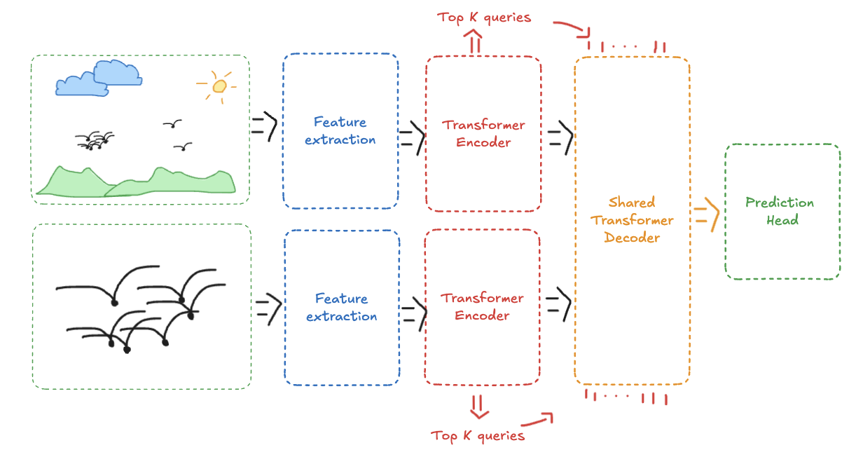
As you can see, each branch has their own backbone, own encoder, and share the decoder. We will be mainly focusing on the encoder/decoder.
Let's say we have run a simple CNN backbone, and output a feature grid which is (this is just for the sake of simplicity, this is essentially useless..).
For one query token at reference point , single head: Input: (dim , e.g. 256).
has shape . This is a learned projection matrix that maps the query token () into the 4 sampling offsets in one shot. The offsets come in x,y offset pairs, explaining our 8 outputs becoming our 4 offsets.
We have a linear layer where we perform: . We now have 4 logits which we pass into the softmax function, resulting in our attention values that sum to 1.
Sample the feature map at each offset location (bilinearly, since the location is continuous), then project it through learned matrix to get the value vectors.
Combine the 4 sampled values into one vector by weighting each with its attention score.
Add the result back to the original token (residual, so it keeps its own information) and normalize.
Pass through a feed-forward network with another residual + norm to finish the encoder block.
Now we have allowed our feature tokens to speak with each other, and learn more about their spatial surroundings. Next step is a very lightweight classification head that will allow us to select our top K queries, based on the "objectness" of our encoder tokens.
Our encoder output can then be denoted as: , where is the total number of tokens (all spatial cells across levels) and each .
Here is a visual overview of the above steps:
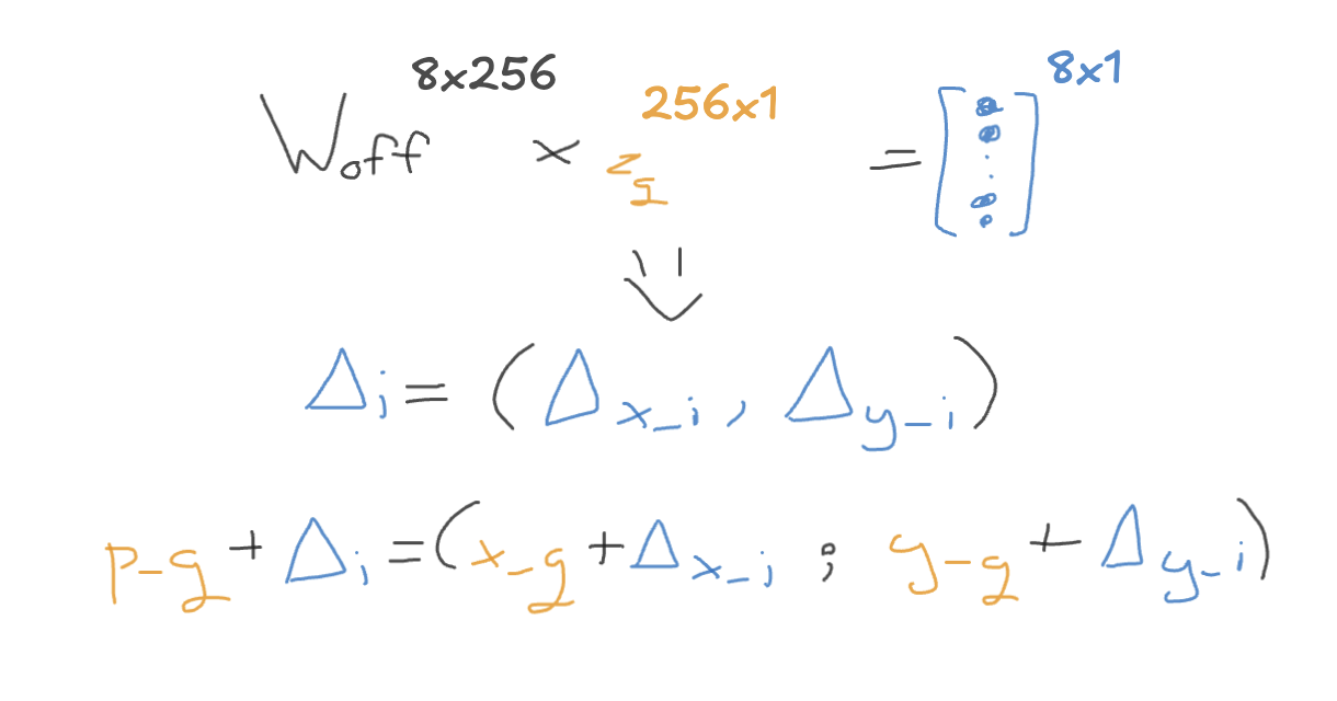
First we calculate our sampling offsets, which are then paired, based on x and y coordinates (as we are just working with point detections, not box coordinates)
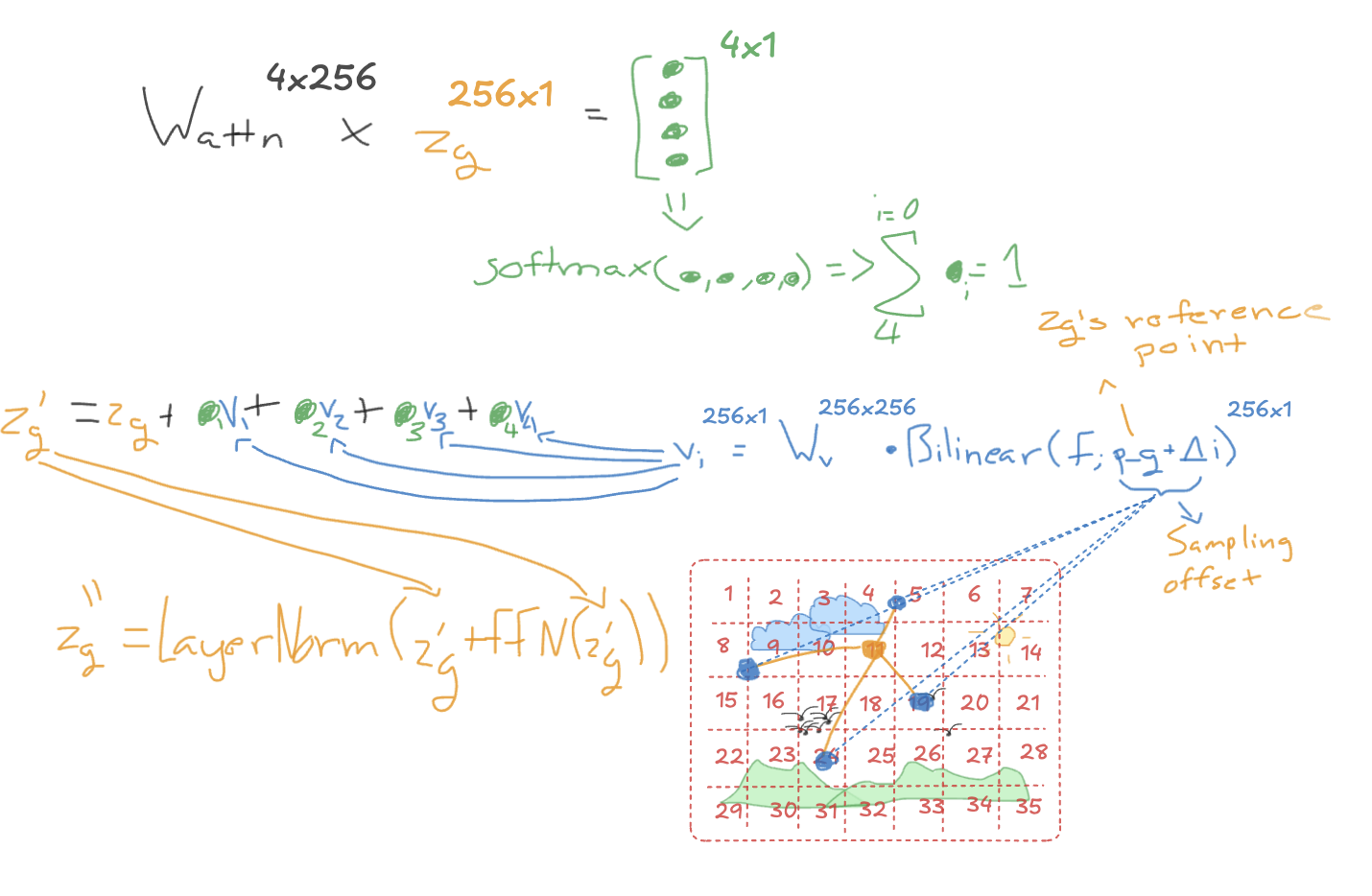
After we have our sampling offsets, we can then move onto to generate our attention values. Then we fetch our sampled token values via interpolation, and project them from our learnt value projection matrix. Now we have our 4 value vectors, which are normalized by our attention values. And these values are at last used to update our base token . Which is then updated by taking its residual into a Layernorm plus its residual through a FFN.
I've color coded it so orange is our base token, and blue are the sampling locations. Green are the attention values which will decide how big an influence each sampled token will have on our base token.
Our bilinear function, is bilinear interpolation, as our sampled location isn't a pixel, it's a continuous location. So what we do, is that we sample the 4 feature cells around our sampled location, and interpolate the value based off the distance from the sampling location and the feature cell, the closer the cell is to the sampled location, the higher influence it will have.
All our encoder tokens are a candidate. We perform a single linear layer across all tokens:
In our example, we will just be using the top 300. So now we select our top 300 encoder tokens to be our queries based off their score.
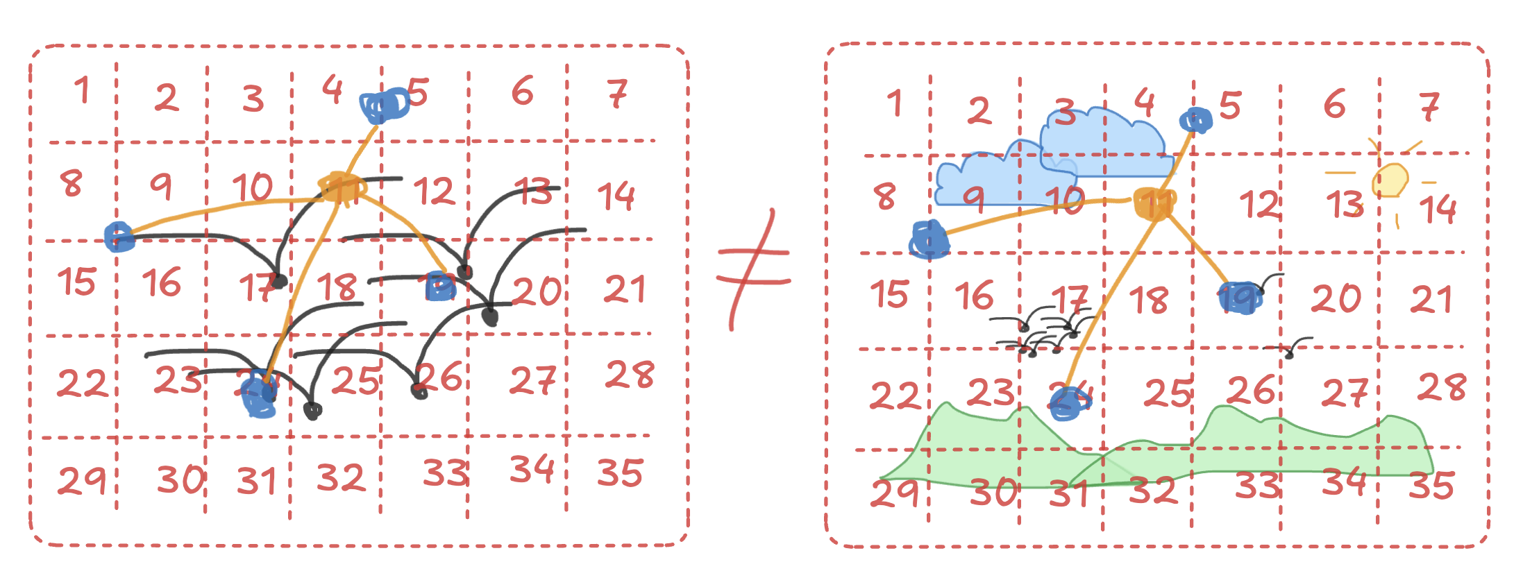
Now the reason why we only share our decoder and not encoder, is because how would the encoder function with these 2 completely different feature grids. As you've seen, our sampling locations have a huge impact on this architecture.
The below image shows how the same sampling locations, will be sampling completely different features.
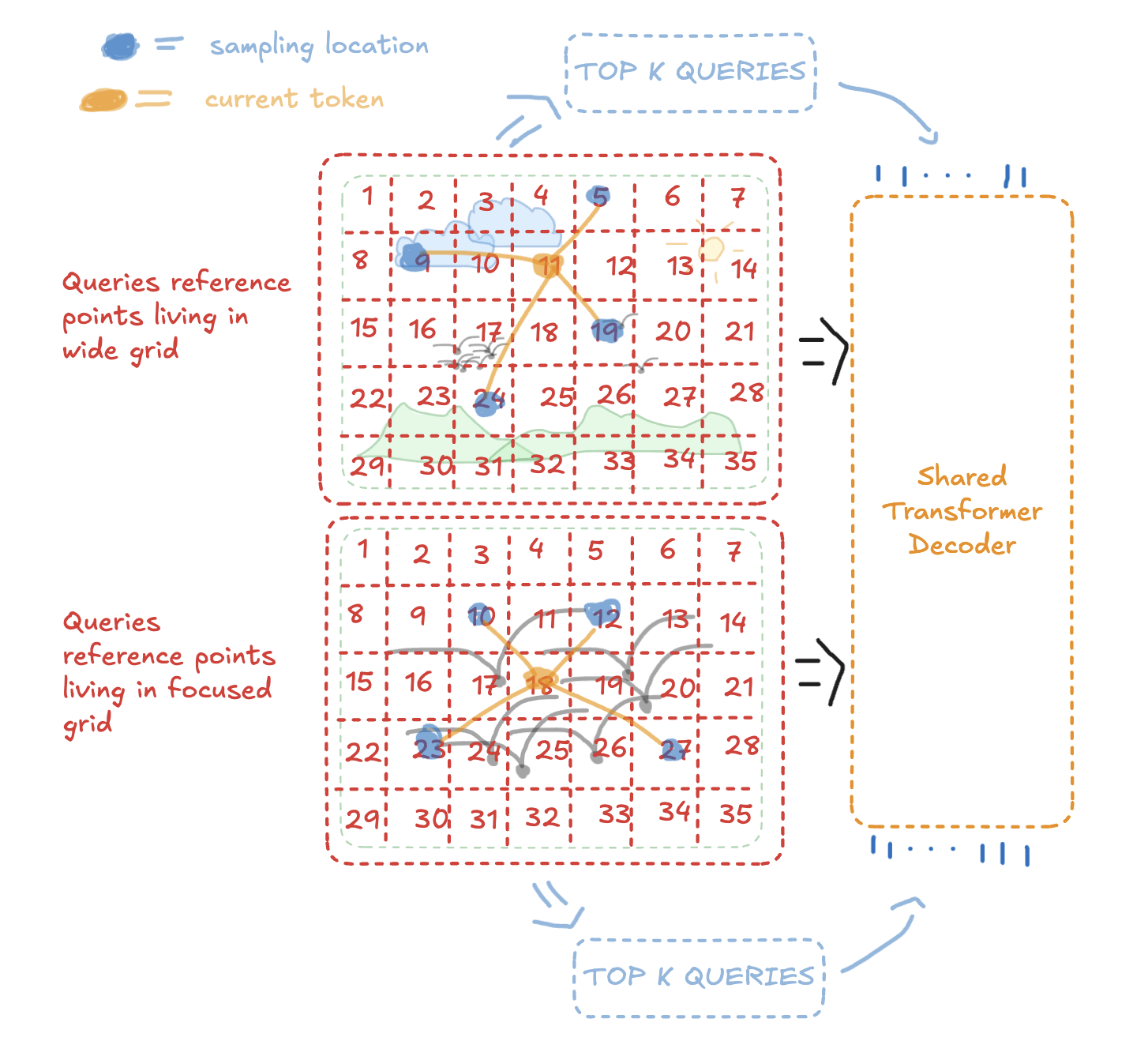
Now onto our decoder. The reason we can share the decoder is due to our reference_point projections.
Here is how is an overview of our decoder:
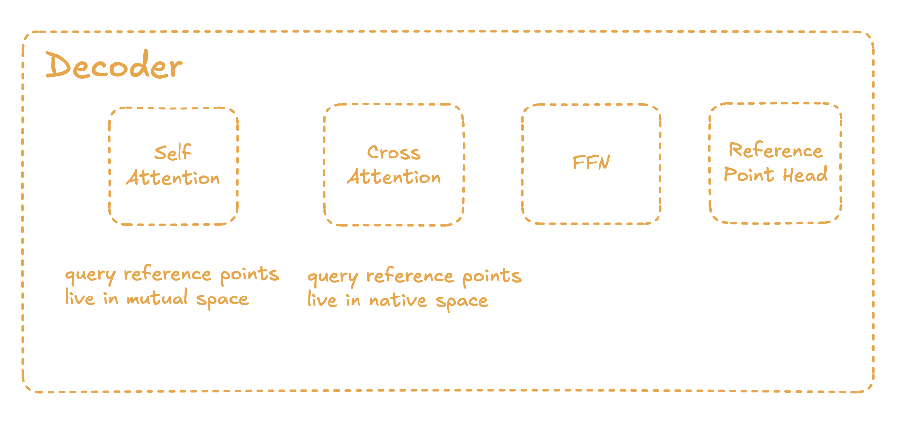
Our first step is self attention between the queries. This is performed in a mutual space. Meaning we are projecting our and into . This will allow our queries to communicate and dedupe with one another.
This self attention is performed via regular attention, not deformable. Meaning all 600 queries will attend to all other 600.
Query content embeddings:
Positional Embeddings projected to mutual space:
Add positional info, then project to Q, K, V:
with .
Scaled dot-product attention (every query attends to all 600):
Residual + norm:
Now onto cross attention, where we want our queries to communicate with the encoded grid. Our encoded grid cannot simply, or easily be projected into a mutual space. They both remain in the native space, of wide or focused. What we can instead do, is project our queries to wide, and focused respectively. Allowing the query to extract information from both grids.
Here are the steps for cross attention:
- Project the query's mutual anchor into both frames -> (B, Q, 2 levels, 2)
- Predict offsets + sample K points in wide AND K points in focused, so 2 levels x K sampling locations total
- The attention weights are softmaxed jointly across all 2xK points (one distribution spanning both views, summing to 1)
- Single weighted sum over all of them -> one output vector -> residual/norm
(B, Q, 2 levels, 2)
- B: Batch size
- Q: amount of queries (600; 300 from each view in this example)
- 2 levels : the two views which we have a reference point for each
- 2 : the coordinate pair (x,y)
Now the math is essentially identical to that of our self attention in the encoder. Only difference is that we now sample information from 2 separate input views.
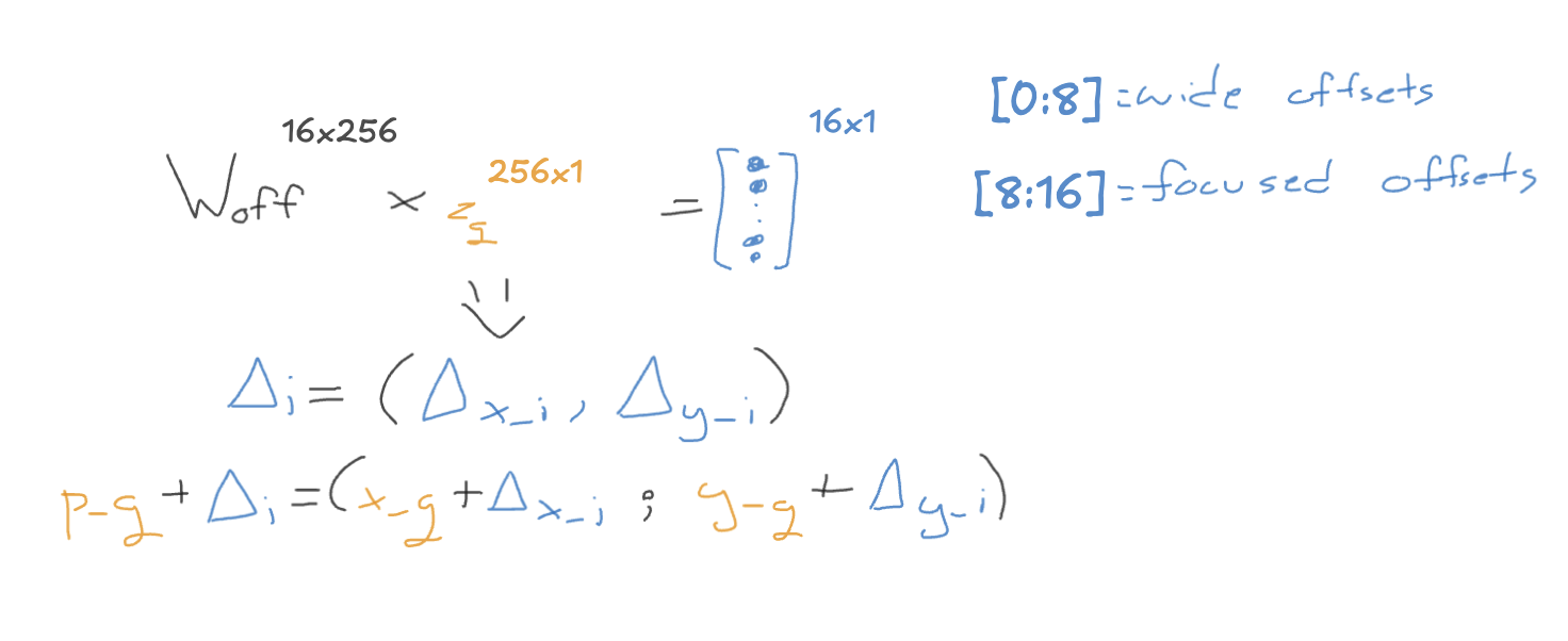
As you can see, our offset matrix has expanded to now . As we now need 8 coordinate pairs, 4 per view.
Now the remaining math is the same, where we apply the offsets to the respective frame, and encode the information from both views onto the query token. Which is visualized below:
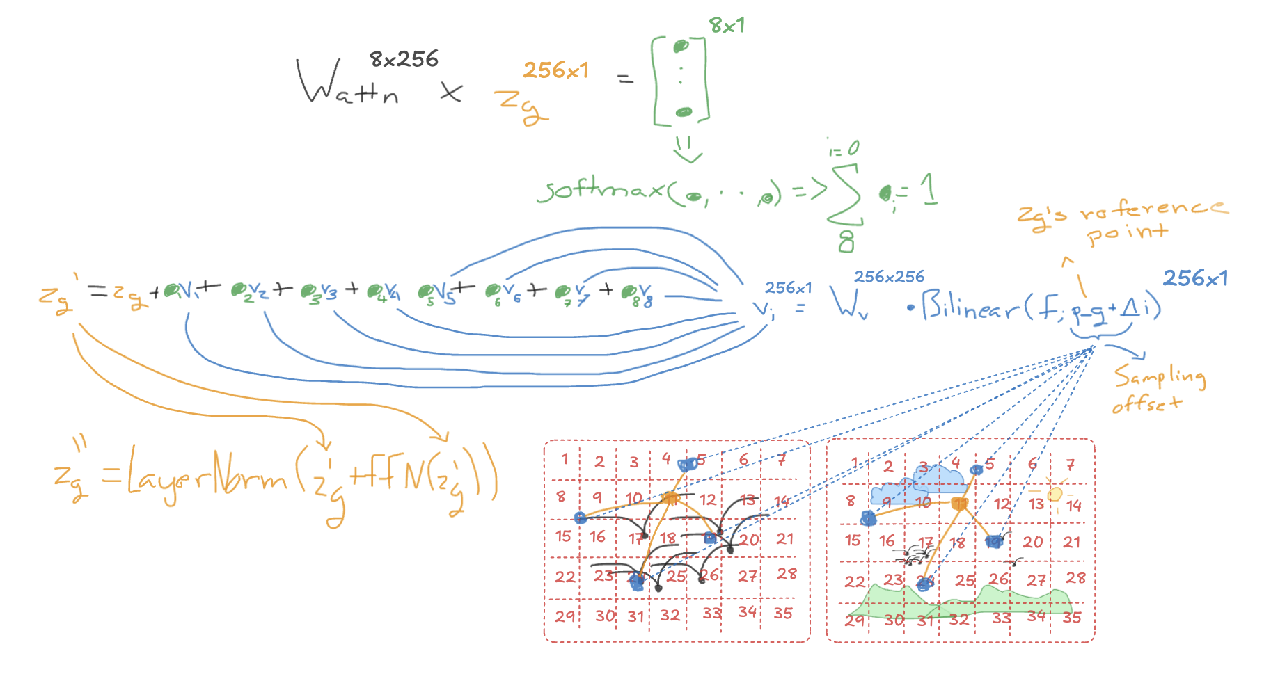
Now our query is extracting information from both views, where one allows it to get full grid information and ensure no bird is overseen, and whilst also allowing the queries to extract from a more refined resolution when birds are clusted, and occlusion occurs.
After the full decoder layer (self-attention → cross-attention → FFN), a per-layer point head reads the refined query content and predicts a small correction to the reference point. Let be the query content output by layer , and $p^{(l)} be the mutual space reference point going into that layer:
where is the sigmoid and the inverse sigmoid (logit).
Now we have the reference point for the next layer, which will now be sampling from a more refined location, repeating this process until we have our final queries, which we will be performing object detection with.
Now we can use our final query embeddings to detect our objects:
Classification (score):
Localization (point) : the refined reference point itself:
So each query outputs . Being a location and a confidence, both derived from the content embedding, which extracted information from both input views.