JEPA

Joint embedding predictive architecture; discussed paper: https://openreview.net/pdf?id=BZ5a1r-kVsf

1. Introduction

The paper this article will be discussing is the paper from Yann Lecun. Yann often speaks on an architecture which can model the world more precisely & effectively. He often speaks on the data hungry nature of RL and LLMS.

He attempts writing this paper whilst answering three main questions:

• How can machines learn to represent the world, learn to predict, and learn to act

largely by observation?

• How can machine reason and plan in ways that are compatible with gradient-based

learning?

• How can machines learn to represent percepts and action plans in a hierarchical manner, at multiple levels of abstraction, and multiple time scales?

I have split this article, in the same structure as Yann does, however more concisely :)

2. A Model Architecture for Autonomous Intelligence

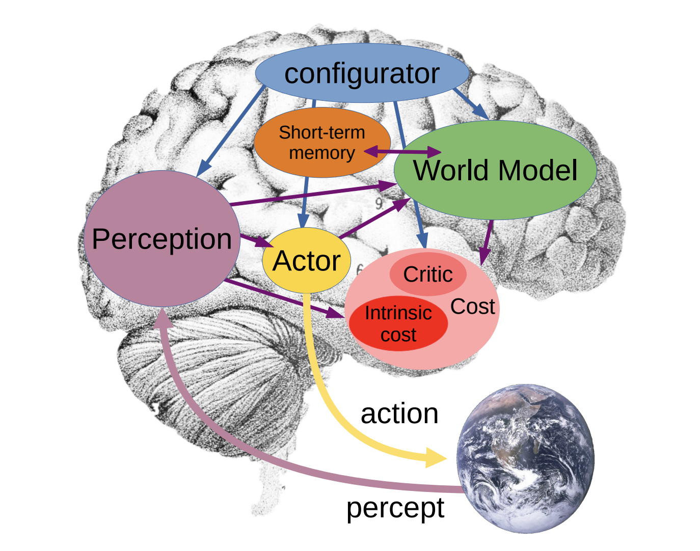
A world model, can be understood as ones perception of its surroundings. World models are interacted with mostly through observation before interaction. The above image, shows the overall architecture of jepa, which is broken down into some modules:

• Perception: Responsible for estimating the current state of the world.
• Actor: Actor is responsible for predicting an optimal set of action sequences, which then only applies the first action from the most optimal sequence.
• World Model: The world model then takes these action inputs from the actor, and predicts the outcomes of the world where these actions are applied.
• Short-term memory: Responsible for keeping track of the current state of the world, and previous actions, as well as the respective intrinsic costs.
• Cost: The cost module outputs a single scalar which is referred to as "energy." There are two sub modules:
• Configurator: A bit of hand waving here, but the configurator model takes input from all other modules. Then configuring them to align with the current task.

Architecture of non-generative predictive world-models

Now let's begin getting a bit more into the specifics. First we need to understand what we are encoding, what our goal is, and how we achieve it.

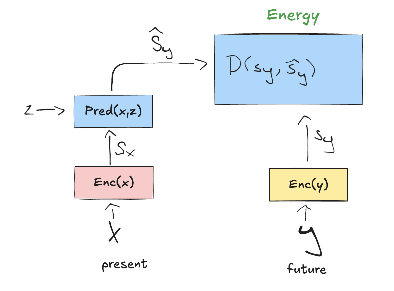
• Prediction happens in representation space, not pixel space, which is what makes this non-generative. This allows the model to ignore unpredicatable detail (pixel textures for example) and focus only on what matters.

• Note on z: it captures what can't be predicted from x (e.g. a car turning left/right)

Intuition: we are encoding our present and future, where we then predict a realistic future, given the encoded present, alongside our variable "z". From there we merge both branches, calculating the energy, which tells us how off we are in our prediction/representation of the future.

There are many losses/regularization steps in this architecture, which will be slowly introduced in this article.

Yann presents this model in two modes:

Mode 1

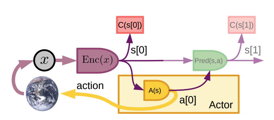
The diagram above shows on step of Mode-1, which is our purely reactive perception-action loop. I will sketch out the steps in order:

1. Perceive: encodes our raw input x into a state representation .

1. Act: The policy module directly maps to an action . This is done with no planning or lookahead, purely reactive.

1. Cost check: computes the energy, informing the model how costly or uncomfortable the current state is.

1. Perform action: is sent out to the environment (the arrow pointing back to the globe), which changes the world, then produces a new percept x.

1. Optional world model update: can predict the next state s[1] from (s[0], a[0]), just so our predictor can be trained again what the actual next percept is. This is simply for training purposes.

Now onto our 2nd mode, which is forward looking.

Mode 2

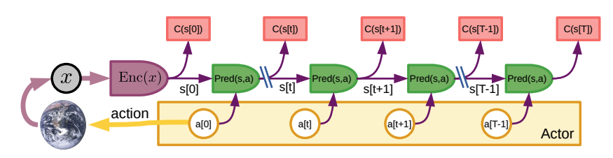
Now our steps are a bit more intertwined:

1. Perceive: produces the current state .

1. Propose actions: The actor now proposes a whole sequence of actions: a[0], a[t], a[t+1], ..., a[T-1], not just 1 reactive action

1. Simulate forward: The world model is chained recursively. Each predicted state s[t+1] is generated from the previous predicted state and action. Meaning it is imagining the future without touching the real world.

1. Evaluate: Each imagined state gets a cost , which is our energy scalar. These energies are then summed into a total predicted cost for the whole sequence.

1. Optimize: Since everything is differentiable, gradients of total cost flow back through the chain of predictors (which wouldn't be possible for mode 1 which relies on polling the real world which isn't differentiable) to the action variables, letting the actor iteratively refine the action equence to minimize total future cost (this is the receding horizon MPC idea).

1. Act: Only the first ation (or first few) from the optimized sequence is actually sent to the world. These actions are then stored to the short term memory module, alongside the respective states.

The key contrast between this mode with mode-1 is that the world model is doing the heavy lifting before acting. It's used for actual planning/lookahead, not just passive training. This is more powerful, but of course a lot more computationally heavy, as for every predicted action, we will be predicting world estimates, and refining our actions based off of it, at every inference.

Let's understand our cost function better:

Reasoning as Energy Minimization

You might think that the cost function also takes the real world as input, and compares the predicted world state from the world model, with the true world. That is not correct.

Cost Module as the Driver of Behavior

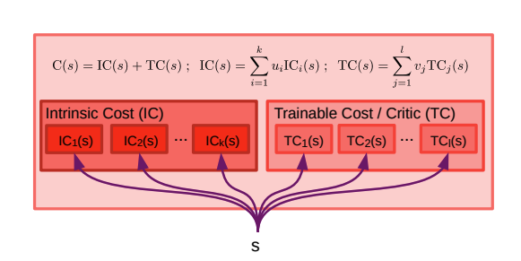
Our energy, is the summation between our intrinsic cost, and our trainable critic. The intrnsic cost is hardwired, not learned. Think of it as inbuilt signals, such as "battery low = bad." And on the other hand we have our trainable critic, which is taught to predict future intrnsic costs from state, using stored (state, cost) pairs from past experiences.

The math is written as follows.

• : the i-th hardwired intrnsic drive (pain, hunger, danger, etc.), fixed function

• : the fixed weight for drive i

• : the j-th trainable critic submodule, learned to predict future intrinsic cost

• : weight for critic submodule j

• : both modulated by the configurator to shift focus between subgoals

The intrinsic costs can all look different. They output scalars (a discomfort value for per drive).

For example:

^ scalar rising as energy drops

^ scalar rising with excess force

As you can see, these are simple hardwired formulas, which can be used as thresholds or indicators. There are no learned parameters.

While IC calculates the current state discomfort, our TC is trained to predict the future discomfort which our IC will experience. It can be seen as a small neural net that takes the current states and outputs a scalar, which is our predicted danger/cost coming steps ahead.

It's trained on stored memory pairs to match the actual future intrinsic cost:

Our stroed memory is the short-term memory module, which is used during planning: (time, state intrinsic cost) = (, , IC(s_{\tau})).

For training TC, we retrieve a past state , and its intrnsic cost at a later time . This "state now, cost later" pair is what TC learns to predict.

This split makes sense, as we want to have fixed "instincts" for our agent. Which can't be drifted during learning. While TC adapts with experience. Very synonymous with how we humans operate. The TC is used to let the agent estimate long term cost heaply without running the expensive world-model rollotu for every step. Which can be seen as an anticipation shortcut for planning.

Training the Critic

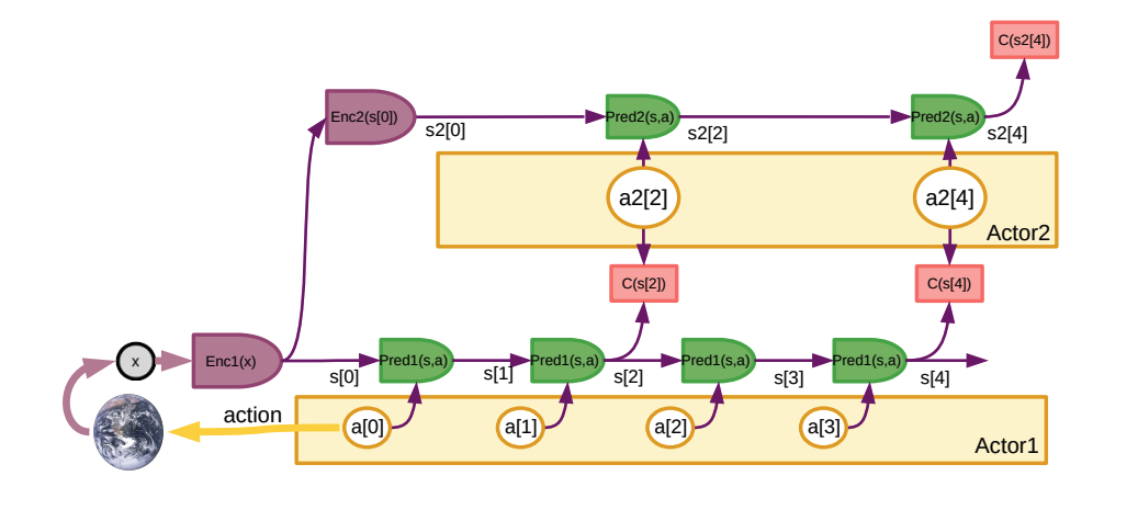
3. Designing and Training the World Model

3.1 Self Supervised Learning

3.2 Handling Uncertainty with Latent Variables

3.3 Training Energy-Based Models

Now onto our non-contrastive technique, which are one of the more novel sections in the paper. Recall that JEPA is trained by pushing down energy, meaning the prediction error beetween and ; on real data pairs. There is some danger in this though, which is that there is nothing stopping the model from cheating.

Bringing us to, the collapse problem. Imagine both encoders (the encoder for our input x, the before state, and our after state, y, which we are learning to predict) learn to ouput a constant vector, ignoring their inputs entirely. Then = always, the prediction is perfect, and the energy will subsequently be 0 everywhere. This is called collapse, when our representations are completely useless, and preventing this collapse is a large challenge of training JEPA.

There are two well known solutions:

1. Constrastive methods: push energy down on real pairs, and up on "negative" pairs (hallucinated incompatible samples). The problem is that in high dimensional representation space, you need an exponential number of negatives to cover every direction the energy could wrongly stay low. This is the curse of dimensionality, and it's why Lecun argues against constastive methods in the long run.

• F.ex. a real pair could be x showing a trolley crusing down some tracks, and y could be the trolley stationing and picking up passangers. That would be a real pair, where we manually tell the model to lower energy. However a bad pair could be x showing the same trolley and y being a banana doing the splits. Not much hardwiring done here, simply mix some training data, so the pairs don't match, and the model will learn the contrast.

1. Non-Contrastive methods: no negatives needed at all. Instead of plugging holes in the energy landscape with our bad pairs, we directly shrink the volumne of low-energy space, so it "wraps" tightly around the real data. This dodges the curse of dimensionality, which is why LeCun favors this route.

As implied, JEPA is trained via non-contrastive methods, to pull this off, it's trained under 4 criteria:

1. Maximize the information content of about x
2. Maxmize the information content of about y
3. Make easily predictable from
4. Minimize the information content of the latent

Criteria 1 & 2 are what prevent our collapse from earlier. If the encoders are forced to carry real information about their inputs, they can't just output a constant. Criterion 3 is simply our prediction ojective (the energy term). Criterion 4 stops a sneaker form of cheating: if the latent z carries too much information, the predictor can just smuggle the answer through it (set ) and collapse the landscape again. So we throttle by making it discrete, low-dimensional, sparse, or noisy.

VICReg

VICReg is the concrete recipe for criteria 1 & 2. The intuition is to keep a representation informative, make sure (a) every dimension actually varies (nothing is constant), and (b) the dimensions aren't just copies of one another.

We map and through an expander network into higher dimensional embeddings, then compute 3 loss terms over a batch:

Variance: keep each dimension's standard deviation above a threshold , so no dimension collapses to a constant:

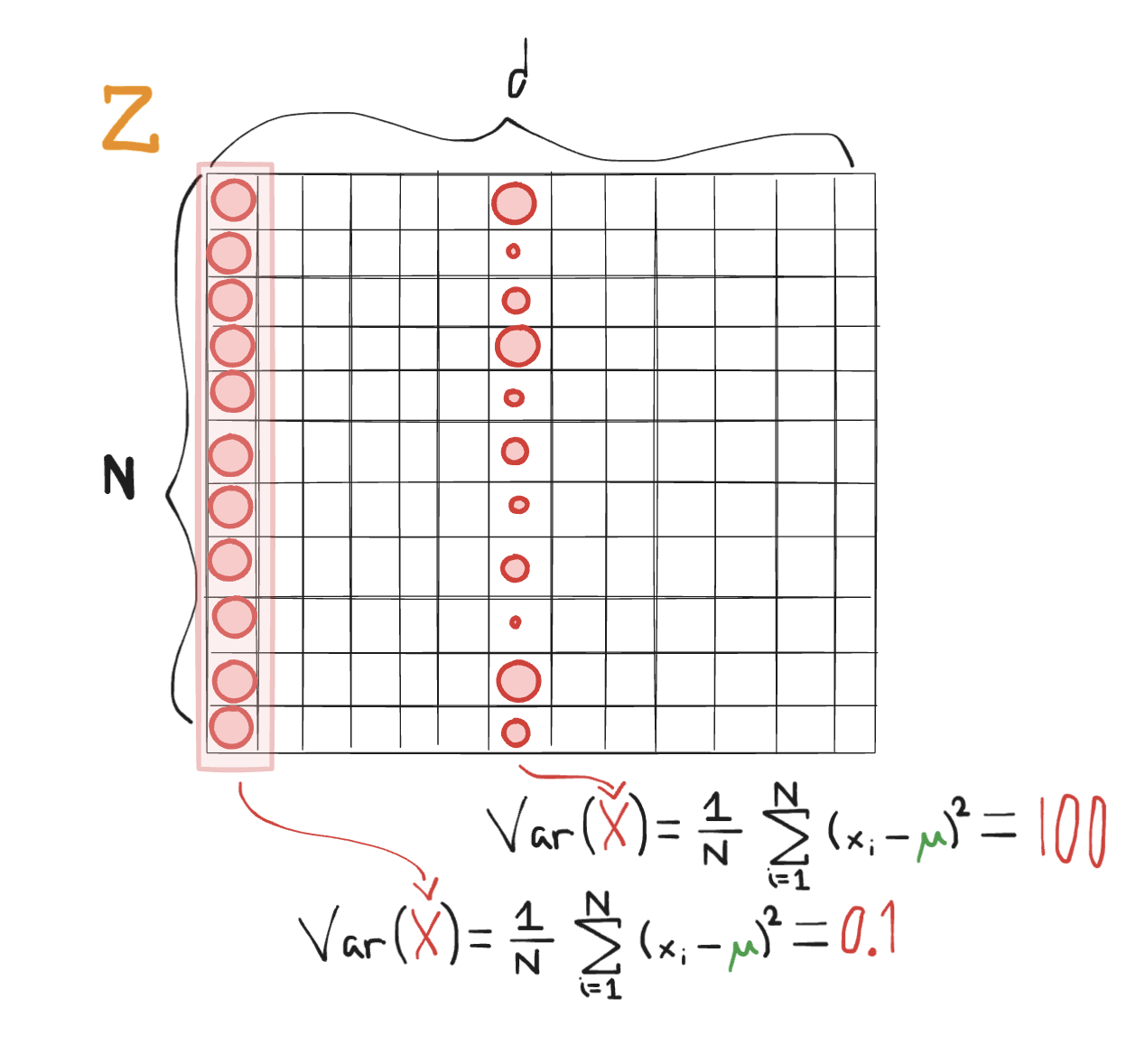
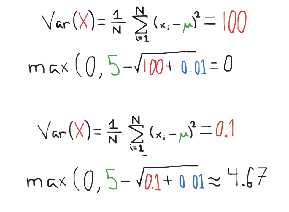
You can envision this as Z being our embedding matrix, every row is an embedding, with d columns. This function ensures that every column is variant, and if not then it is punished. selects dimension j from all rows . We take the variance from that dimension, add a small safety margin epsilon, then subtract the value from our threshold . If our variance is low, the value will be high, meaning it will be over 0, and the penalty will be that value. Values of 0 and under naturally won't punish the model.

Some visuzalition below:

Invariance: this is criterion 3, the prediction error pulling the two branches together:

This is simply taking our two branches embeddings across our batch N. For each sample i, we take the predicted embedding and the target embedding and take the squared difference. We then find the mean of between all samples across the batch. This then punishes the model when the two are very different, far away in dimensionality. Which eases the learning of the model (criteria 3).

Covariance: we push the off-diagonal entries of the covariance matrix toward zero, decorrelating the dimensions so each carries different information:

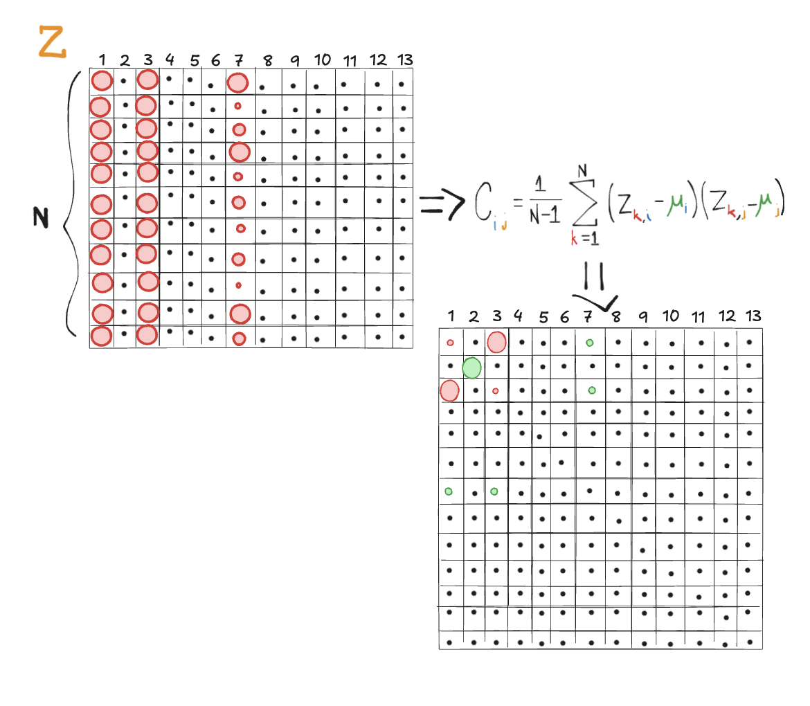
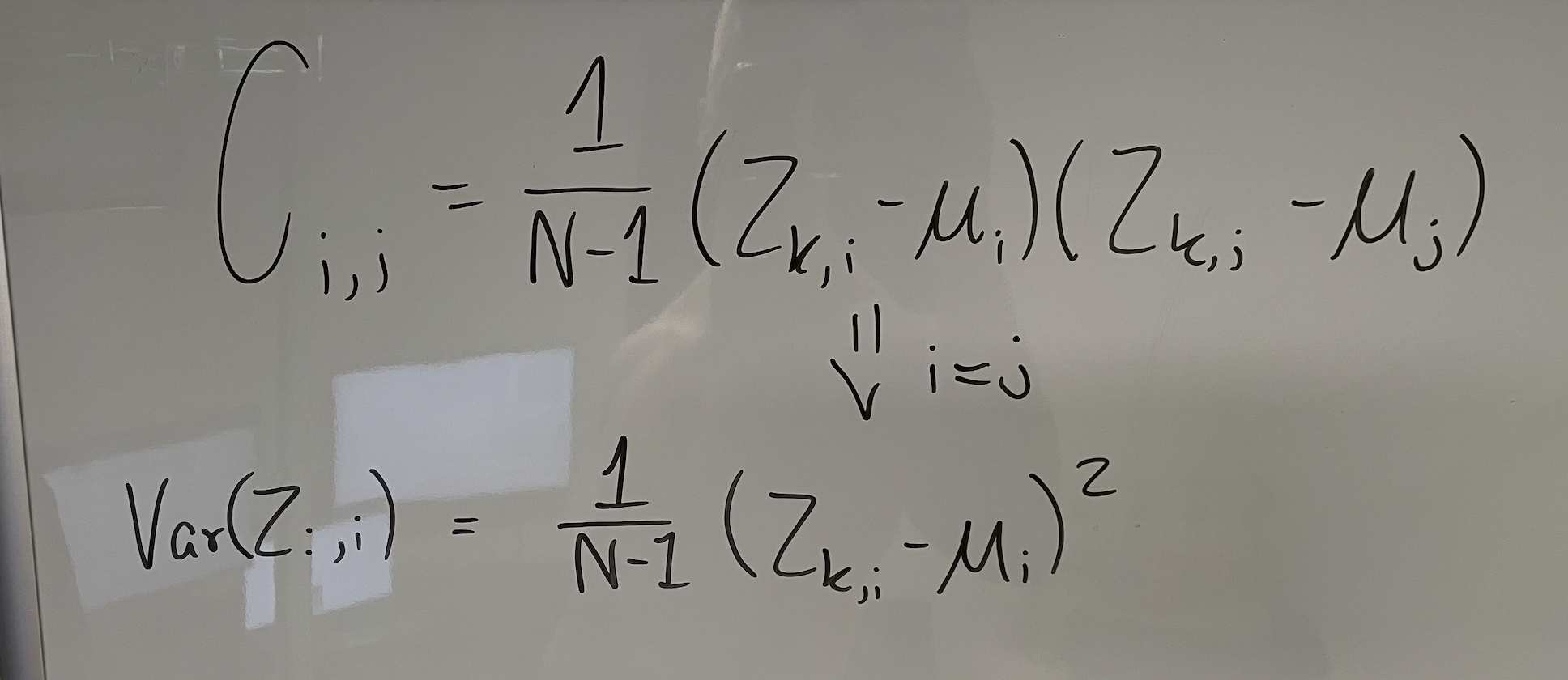
Here is a drawing with a concrete example. Keep in mind that the covariance equation given the same dimension, is the exact same as calculating the variance.

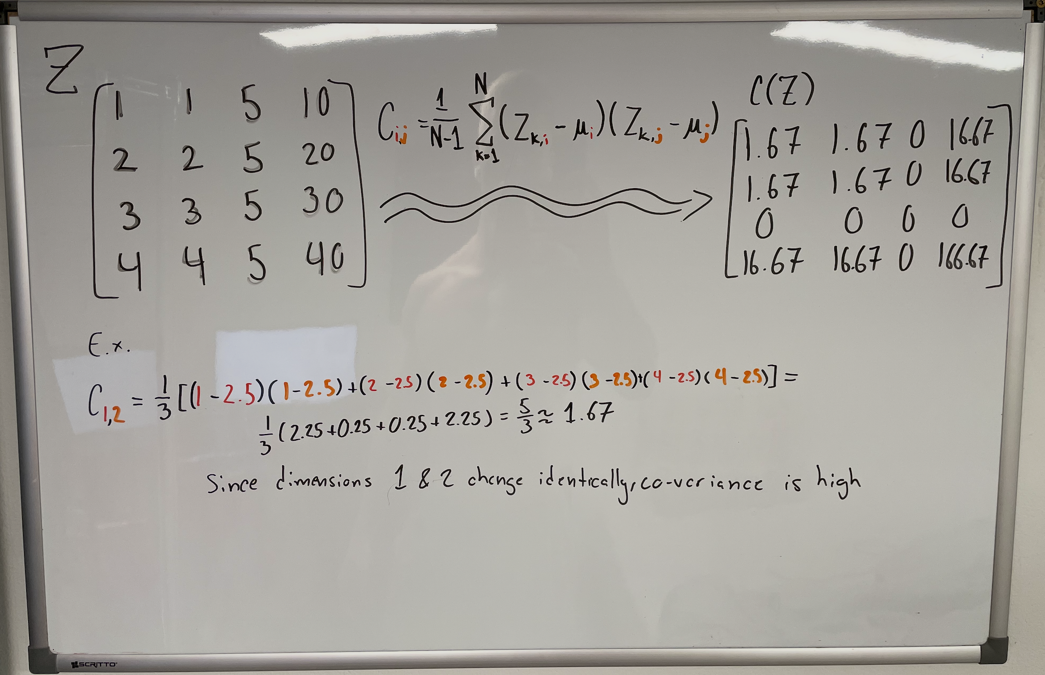
• High positive covariance means they move in the same direction. Meaning in our diagonal offsets, we want those values to be low, so the dimensions represent different information. Whereas the diagonal values should be high as we want high variance (and the covariance of the same dimension tells us the variance.)

3.3 Handling Uncertainty with latent variables

Total Loss

The total loss is a weighted sum of the 3, applied to both branches:

Traditional contrastive methods are sample-contrastive, meaning they push apart different samples, which is exatly what forces you to chase an exponential number of negatives. VICReg is dimension-contrastive, its variance and covariance terms push apart different components of the representation over a batch. It never touches a single negative sample. It just insists that each dimensino varies and that the dimensions stay decorrelated, and that in itself is enough to prevent collapse.

3.4 Joint Embedding Predctive Architecture (JEPA)

3.5 Training a JEPA

3.5 Hierarchical JEPA (H-JEPA)

3.6 Hierarchical Planning

3.6 Handling Uncertainty

3.7 Keeping track of the state of the world

3.8 Data Strams

4. Designing and Training the Actor

5. Designing the Configurator

Hierarchical Planning