NeRF: Neural Radiance Fields

Scene as a function

NeRF: scene as a function

NeRF stores the scene in a neural network. If it's given a 3D point , and a viewing direction , it will return a density (how much stuff is there) and a colour :

To colour a pixel, we shoot a ray from a camera through it and add up the light along it. This is volume rendering:

is the trasnmittance, which means the fraction of light that makes it from depth t back to the camera without being blocked. In practice the integral is approcimated with N samples spaced apart:

(Note: Gaussian splatting uses exactly this formula, except the \alpha_i comes from elsewhere)

weighted-rays

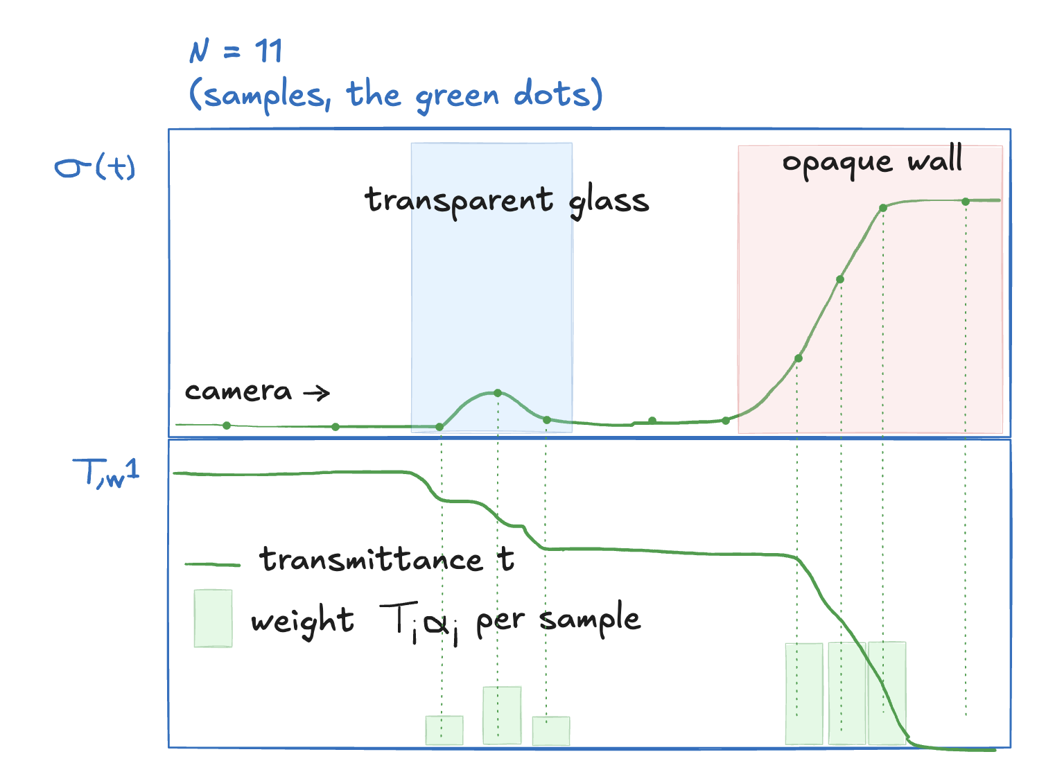
Above I have visualied a ray that has 11 sampling points. In this given image, the ray passes through a transparent blue glass, finally landing onto a red opaque wall. Which can be seen on the above container. In the below container I visualize our transmittance, which drops every time it passes a surface. It has a weight per sample. As you can see, the weight is 0 in the samples that have no surface contact, and increase with the opaqueness of the surface.

The final color of this pixel is then the weighted sum of the sample colours. Which in this case would be a red pixel, with a slight blue tint.

Something that stumbled me intuitively, is how we could perform this task without knowing the actual depth and distance from camera to surface. This is of course not necessary, as we are working with the concatenation of multiple input views. The network commits to one 3d position for the wall, shared by all views. If that depth is wrong, the wall lines up in one camera but lands on the wrong pixels in others, so the loss there is high. Gradient descent moves the density until every view agrees, so depth is never given. It is created by being consistent across the different views.

Example

I will run through a worked example, to make sense of it.

formula · variables · role · learned? · : camera centre; : unit direction through the pixel; : distance along the ray · pixel → ray; samples between near/far bounds · no (from camera pose + intrinsics) · : network weights; : 3D point; : density; : RGB colour · queried once per sample · yes, is the only learned thing · : true pixel colour along the ray · ideal physics; never computed · no · : fraction of light still reaching the camera from depth · over one slice gives , the basis for · no · : distance to next sample; : opacity of slice · fraction of light stopped at sample · no · : light left when reaching sample · discrete transmittance · no · : weight of sample ; : rendered pixel · the colour actually rendered · no, gradients flow through it · : the pixel in the real photo · compares render with photo, drives learning · no

As you can see, most formulas are not learned, except for our Function, which given a 3d point, and the unit direction, we then output a RGB color, and density (sigma). There are then some formulas where our gradients flow through them in backpropagation, for example our predicted pixel, which is used to be compareed to our ground truth pixel.

Here are some variables to start our example out with:

We have 1 ray with 3 samples, [1,2,3].

Sample 1:

In the first sample, there is no surface, just air, therefore the density is 0, meaning our prediction for color , from our network function is empty. The opacity () is then 0, our Transmittance is 1, as it tells us the light left when reaching sample i, which in this case is only light. And our weight () which is our Transmittance times opacity, which then gives 0. Simple enough.

Sample 2:

Our ray now hits glass, density is predicted to be 0.5, color blue, opacity 0.39, transmittance still 1, and the weight, being our opacity times transmittance is then 0.39.

If you wonder how come the transmittance is 1, given we reach a surface, then recall the formula, , where i is 2, therefore j only takes sample 1 into account, so 1 - opacity from sample 1, which is , therefore the transmittance remains 1, as it doesn't include the current sample.

Sample 3:

We hit our red opaque wall, density is predicted to be the value 3, color red, opacity 0.95, transmittance 0.61, weight 0.58.

The pixel: , and the weights plus leftover light add up to 1.

Neither the blue glass or red wall contains green, therefore the color green only comes from our white background. Below you will see the value of for red and for blue, and that is due to the background being added to them, here is a very simple table that explains that logic:

source · weight · colour (R, G, B) · contribution glass · 0.39 · (0, 0, 1) · (0, 0, 0.39) wall · 0.58 · (1, 0, 0) · (0.58, 0, 0) background (white) · 0.03 · (1, 1, 1) · (0.03, 0.03, 0.03) (sum) · 1.00 · · (0.61, 0.03, 0.42)

If the photo's pixel is pure red (1, 0, 0), then L = (0.61−1)² + 0.03² + 0.42² ≈ 0.33. Backprop lowers the glass's density or shifts its colour toward red; other views decide which.

channel · · · R · 0.61 · 1 · 0.152 G · 0.03 · 0 · 0.001 B · 0.42 · 0 · 0.176 ** · · · ≈ 0.33**

Training Loop

A random batch of n rays from random photos are then rendered, we then calculate the loss, perform Adam step.

So rays from random photos render loss Adam step (gradient descent)

Network

A plain MLP (multi-layer perceptron) few raw (8 layers x 256 neurons). is computed from x only, then is fed in for the color. Which is why geometry is the same regardless of angle, while the reflections can change.

Positional Encoding:

An MLP fed raw (x,y,z) can only learn blurry functions. Whereas if we expand each coordinate into sin/cos at many frequencies lets it represent sharp detail. This is on of the key tricks this architecture has.

Hierarchical sampling:

64 coarse ray samples find roughly where the surface is (high weights), then 128 fine samples go there. It ties back to my explanation on how the network knows the depth of objects.

Where the poses come from:

COLMAP / structure-from-motion, plus the near and far bounds

Limitations:

640,000 rays x 192 samples = 122,880,000 network evaluations per 800x800 frame, which means 1-2 days of training (depending on the hardware of course) per scene and seconds per frame. Most samples are wasted on empty space.

Not long after (3 years) the publishing of NeRF, another architecture, making use of gaussian splatting was released, which solves the above limitations, which you can read more about here: