Salience DETR

Intuition to: https://arxiv.org/pdf/2403.16131

Salience DETR builds off of Dino-Detr. Which is an accurate detection transformer architecture, making use of DAG (dynamic anchor generation), with two-stage query selection, as well as CDN (Constrastive denoising) as an auxilliary loss, alongside LFT (Look Forward Twice) within the decoder layers, but these specifics are irrelevant to this article.

Salience DETR helps our architecture becoming more performant, as well as boosting the accuracy by a slight margin.

Salience DETR is an improvement from like-minded architectures, such as Sparse-Detr, and Focus-Detr. These architectures focus on refining which tokens should be performing attention in the encoder, to save computation, and avoid encoding redundancy across background tokens.

The increase of queries helps the performance of Dino-Detr, which is visualized below in Figure 1. However with this slight boost in performance, there comes a large redundancy in the queries, where the queries quickly bundle onto the larger objects. Which is also an issue, introduced by scale bias.

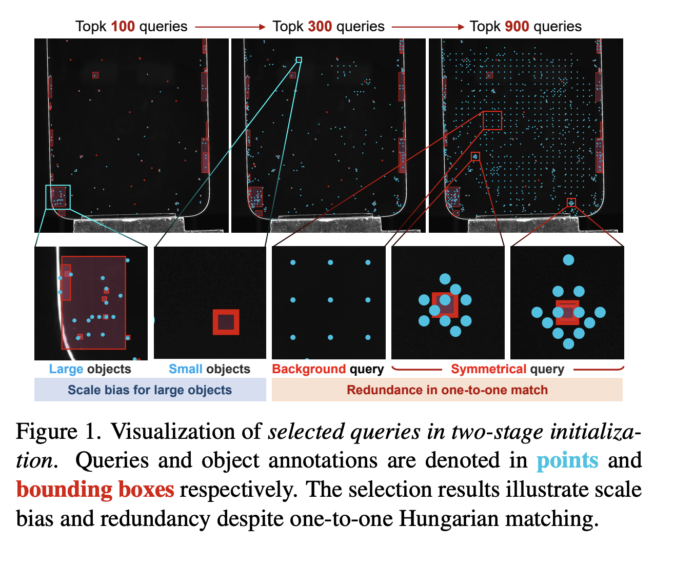
visualization-of-selected-queries-in-two-stage-intialization

There are 2 main issues which Salience-Detr works on:

Encoding Redundancy: Background tokens being encoded with information, which could be called as a waste of compute

Selection Redundancy: The tokens selected as decoder queries don't map 1:1 to objects. Many pile onto one object.

Encoding Redundancy

The encoding redundancy is already attempted to be resolved by other architectures, as aforementioned: Focus & Sparse DETR. However, those 2, don't take scale bias into account. We adress this issue via our salience score:

So instead of our foreground and background score being a discrete values of {0,1}, they are then continuous. By diving with the w and h we resolve the scale issue. As we begin decaying the target value the further from the center of the object we move. An example of this can be seen below.

top-5-query-visualization

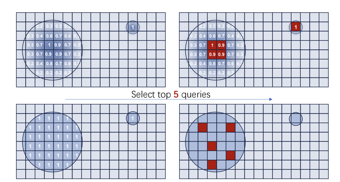
The above row is an example of Salience-Detr where the target value decays the further off-center we move, whereas in the regular query-filtering setup in the row below, we simply have our discrete values of {0,1}, of either foreground or background. This assists our encoder redundancy, as our query filtering is now less biased towards bigger objects, allowing us to have a larger confidence when we pick the ratio of filtered tokens. As we are now more confident our smaller objects are included in the top-fraction of tokens we want to perform attention with.

The top token fraction can attend to the entire grid, including the background tokens, the background tokens aren't removed the grid, we simply don't perform attention with them. Every layer can use a different ratio of top token candidates.

Selection Redundancy

Our selection redundancy is mainly adressed via our NMS, performed after our top-k-query proposal.

Concrete example:

We create a box per proposal (cell at row r, col c, paper Eq. 11):

NMS: sort by score descending, keep the top proposal box -> drop any remaining box with IoU(kept, -> repeat on survivors.

Example: (), 3 proposals -> 2 on one car, 1 on a football:

table-example-of-salience-nms

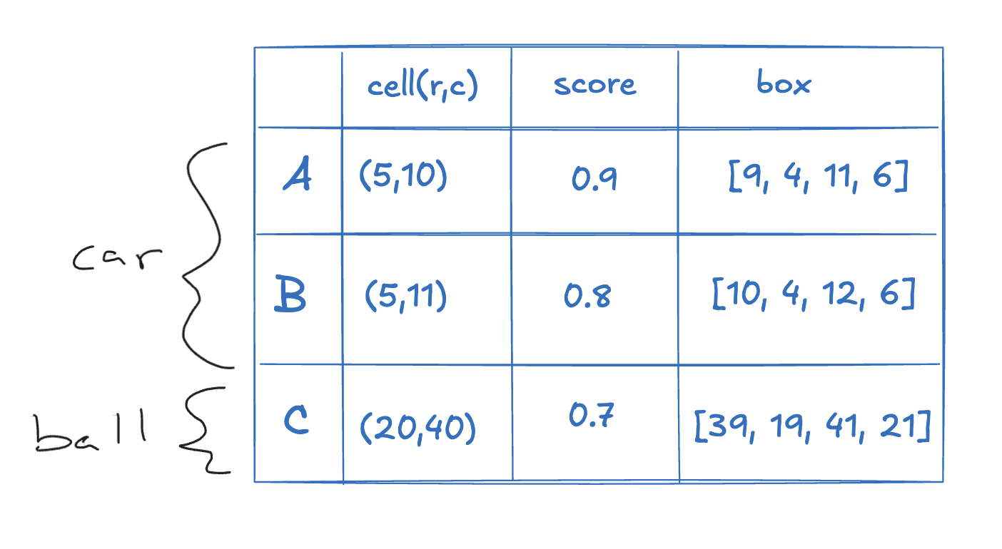
Keep A (highest score).

IoU(A, B)

IoU(A, C)

The negative intermediates in step 3 are the gap between the boxes, our discards them.

This might seem a bit counterintuitive, that we are discarding queries from objects, as it could be information which the model could learn more about the object. But keep in mind, that the box is only a 2x2 grid, the removed ones are near duplicates (edge adjacent, same spot) which makes them (nearly) redundant. And in our hungarian one-to-one, we are forced only one query per object anyways, so the extra duplicates are forced to be "background." In fact, it could supply a confusing gradient (a query setting on a car being told "you're nothing"). Removing them should stabilize two-stage intialization, that's the paper's whole reason atleast.

We aren't discarding any features either, as the value/keys stay on the full map, and the surviving query cross-attends the object, sampling multiple points from it. Complementary detail is achieved by gathering info by the decoder's attention.

How feature levels are handled

This is a smaller detail, but still interesting and worth mentioning. Our backbone can output feature maps at different resolutions. And our encoder will typically have more than 1 layer. We are working with 2 axes, Encoder Layer and Feature Level.

The paper adresses these 2 axes, with 2 coefficients. Our & are values per encoder layer and feature level. The higher level feature maps, have coarser amounts of tokens, representing a higher semantic representation of our image. So the value of the is higher for the higher levels, and decreases the lower you go. Whereas our encoder layer value, is constant.

Meaning the top-k fraction encoder tokens which we allow to self-attend is , the rest are skipped.