Backpropagation

Intuitive explanation of backpropagation

This article assumes that you have a basic understanding of neural networks, and have an intuition on the structure of layers, neurons, and the activation functions which lay between the layers. As a refresher, you can see below the structure of a NN with an input layer, a hidden layer, and an output layer. The same network we'll use for the worked example later:

neural network, 3 layers

Each neuron contains its own function, where its input x are the output activations of the previous layer. It's a simple function that can be written as:

This value is what we call z, the pre-activation value of our neuron. As you are familiar with neural networks, you would also know the importance of non-linearity in the layers, and this non-linearity typically stems from the use of activation functions. There are various activations that can be used, depending on the task at hand. In our case we will be using a simple ReLU activation between the layers, and at last sigmoid for the output layer, as our example will revolve around binary classification. Our final function per neuron will then look as follows:

The goal of our binary classification model is to classify whether you've had too much to drink or not. Our ground truth label y will be 1, indicating: yes, you have had too much to drink.

The loss function will be the classic squared error. (For a single sample it's just the squared error, the "mean" in MSE comes from averaging over a batch, which we skip here since we're working with one example.)

Let's say the prediction output of our model is 0.4. The error would then be:

Loss would be 0.36. Now, how does our model learn from this error? How does it teach its learnable parameters (in this case being and b)?

dependency chain

In the above visualization you can see the dependency chain of the network. Our prediction is the activation of the last layer, which depends on that layer's logit z, which in turn depends on the previous layer's activation and the current weights. This dependency goes on until the first layer of our network. (One notation note: and refer to the same thing, which is the activation of the last layer. I'll use both below.) Our network needs to learn how to update the weights in each layer so that our prediction aligns itself with the ground truth. The chain rule for this operation is also shown at the end of the visualization, and is stated as follows:

This equation shows how the loss depends on the prediction, which depends on the activation function, which depends on the input logit , which depends on our weights . We use partial derivatives because the loss depends on many parameters. Every weight and every bias, and we wish to influence each one in isolation. The chain for the bias looks as follows:

with (z is linear in b), so

This is how the backpropagation equation looks for the last layer L. And this is where the term "backpropagation" comes into play: we want to use the error gradient of a layer and propagate it backwards to the previous layer. The term which is sent back is:

Now we have 3 equations:

The first equation shows the delta which is propagated backwards to the previous layer. The 2nd equation shows the influence our bias term has on the loss. The 3rd shows the influence our weights have on the loss. Now let's look at our previous layer, L-1.

The previous layer will have a longer chain, as it receives the delta of the layer ahead of it. The chain grows by 2 terms for every layer we move backwards. The entire chain will look as follows:

Now let's break this down in plain english: tells us how the weights of layer L-1 influence its logit, and how its logit influences its activation output. That activation is used as input to layer L's z function, hence the term , which tells us how the activation from layer L-1 influences the z function of layer L, and so on and so forth until we reach .

And respectively the chain for b will be shaped as:

Now what part of this new chain becomes the delta which is propagated back another layer? That would be:

And as aforementioned, it has grown by 2 terms. The partial derivative with respect to simply becomes , since . z is linear in b.

Now let's work back to our original example, of whether you had too much to drink tonight or not. We will be working with the network from the start of the article: an input layer with 2 neurons, a hidden layer with also 2 neurons, and an output layer with a singular neuron.

Since we have 2 neurons in the input layer, we are working with 2 input parameters. Let's say that is your weight in kg, and the amount of units you have drunk.

Let's initialize our network with some random weights and biases:

Hidden layer (layer 1):

Output layer (layer 2):

Now let's walk through the forward pass. For each neuron in the hidden layer, we compute the pre-activation value , and then apply our ReLU activation:

Plugging in our values:

These activations now become the input to our output layer, where we compute and apply the sigmoid:

And there we go, a prediction of 0.40. Our loss is then:

Now time to teach this model from its mistakes. As we have 3 layers, we will be calculating:

Once we have these partials, they determine how we update the weights & biases, via gradient descent:

where is the learning rate. These gradient update functions help our model traverse down the loss surface, which can be visualized as follows:

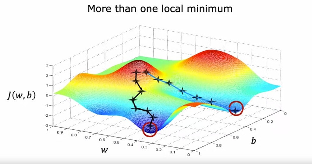
Now back to our example. We have calculated the following terms:

Now let's begin calculating for the last layer L:

For : since , differentiating with respect to gives us the activations of the previous layer:

Now the partial derivative of with respect to . As we know, we are using sigmoid as our activation function for the last layer:

Now our final partial, . Since , differentiating with respect to gives:

Now our final chain looks as follows:

The chain for our bias is even simpler, as its last term is just 1:

And the delta which we propagate back:

Now on to our hidden layer, L-1:

We can insert our delta from the following layer:

Let's begin with the term. Since , differentiating with respect to gives:

Now onto : that is the derivative of our ReLU function, which is simply . Meaning the derivative of ReLU is either 0 or 1, depending on whether z is below or above 0. And if we recall our values:

Both are positive, meaning:

We now have everything to compute the delta for this layer. Note that these products are elementwise, meaning each hidden neuron gets its own share of the error, scaled by its outgoing weight and its ReLU derivative:

Now onto the last term, , which, as we already saw in the layer above, is simply the activations of the previous layer, in this case the raw input:

Since each of the 2 hidden neurons has 2 incoming weights, the weight gradient is a 2x2 matrix: the outer product of the layer's delta and the input.

And for our bias, the last term is 1, so the gradient is just the delta itself:

Now we have calculated the partials for our weights & biases of layer L-1 and L:

Now we can do our gradient updates (learning rate set to 0.01):

Separate result to keep it visually cleaner:

Now let's perform a forward pass with these new values:

Our prediction has gotten far closer to the ground truth label "1", and the loss has subsequently dropped dramatically.

Two things about this result are worth noting.

1. notice how large that jump was for a single step with a small learning rate, that's because our inputs are unnormalized (a raw 70 kg flows straight into the gradients, giving us values like 8.064), which is exactly why in practice we normalize inputs before training.

1. look at hidden neuron 1: its pre-activation went from 2.10 to -3.71, so ReLU now outputs 0, and since the derivative of ReLU at negative values is also 0, no gradient will flow through it in the next backward pass. The neuron has effectively died (which is something GELU can help resolve(ish)). On our toy network this doesn't matter, but it's a real failure mode of ReLU networks, and a nice reminder that the mechanics you just walked through are the same ones that produce these training pathologies at scale.

This has been a very simple example of backpropagation in play.