Unifying Short and Long-Term Tracking with Graph Hierarchies

SUSHI paper analysis: https://arxiv.org/pdf/2212.03038

1. Introduction

This paper (SUSHI) solves the problem of scalability within the task of object tracking. Object tracking consists of difficult problems, such as short-term assocation, which then propogates to helping solve long-term association with occluded objects, which can dissappear and reappear in the scene.

There are many architecturs that solve this task, by yielding a hybrid approach, to solve the short-term and long-term tasks separately. This then leads to quite a substantial amount of engineering overhead.

SUSHI solves this by creating a unified, scalable architecture.

1.1 multi object tracking

Multi-object tracking (MOT) has the goal of identifying the track of an object across time. Simply put: we associate detections across frames. This task can be quite straightforward when association non-occluded detections across a short-term window, by using cues such as motion-based proximity, and local apperance.

However, if the objects begin occluding, then they might not be detected in several frames. Which then forces our model to learn the association through a long-term context. Many architectures solved these short-long term associations separately, becoming hybrid multi-level models.

This then leads to the issue of scalability, since those models cannot deal with long videos. However the graph based models are more robut, but this association through large timespans would naturally lead to very large graphs, which then made the task infeasible computationally and memory-wise.

Second limitation is generality. Different scenarios would require different approaches. A scene of traffic, where cars are similiar, and the frame rate is high, would most likely benefit from a model which makes use of motion-based proximity, whereas if the scene were to be of an aquarium, with many different species of fish, with lower frame-rate, then that scenario would benefit more from an appearance based cue. This then becomes an un-generalized model, which needs to be adapted given the specific task we are trying to solve, leading to handcrafted solutions.

1.2 proposal

SUSHI remains a GNN approach to the task. Where they structure it hierarchically. This allows us to use the same model, for different time scales. This solves our 2 issues:

1. Scalability: the hierarchical structure means its scalable given the varying time-scales of input

1. Generality: the model makes no assumptions on which cues should be used, instead lets the model learn which cues are most benefitial

Strong tracker, with a Unified solution across timespans, and good Scalibility thanks to its HIerarchical nature = SUSHI

SUSHI as mentioned, is a graph method. Where for each level of the hiearchy, it takes as input the formed tracklets from the previous level. Meaning, as the number of tracklets go down, the further up the hiearchy we go, the wider temporal context we go.

SUSHI is given object detections for a frame, and its task is then to perform data association by linking object detections into trajectories. The detection is given the bounding box coordinates, its image region, and timestamp.

Each trajectory is given by its set of detection , being the number of object detections, or trajectory length.

Sushi models data association via an undirected graph where each node corresponds to an object detection, i.e. . Edges represent association hypotheses across the objects at different frames. . Our time ordered track with can be represented as a path in given by its edges . Therefore, our edges can be classified into correct hypotheses if for some , then we can denote or incorrect otherwise. Given a set of edge predictions or costs, . This framing allows us to cast our data association as edge classification.

2. SUSHI architecture

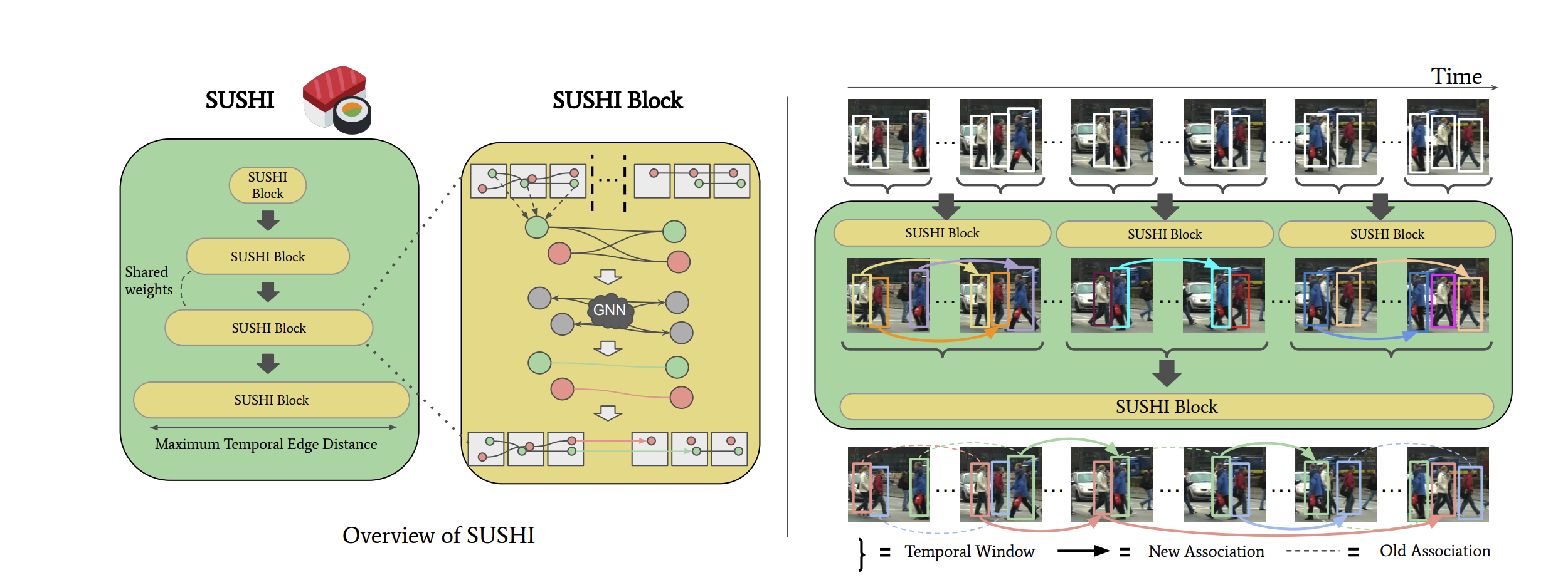
Sushi consists of jointly trained SUSHI blocks, that operate over our video clip. It starts from the inital per-frame object detections (which we refer to as tracklets of length 1 from here on out), each SUSHI block learns to merge tracklets from the previous level into longer ones.

Every node and edge has an associated embedding, our encoding position, appearance, and motion cues, which are then propoagated through our graph. After several of these message-passing steps, our edge embeddings are then classified into correctn and incorrect hypotheses, which then yields a new set of longer tracklets. And as mentioned, the further up we go into the hiearchy, the more temporal ground we cover.

Below is a fine depiction of the architecture:

2.1 constructing the hierarchy of tracking graphs

There are some limitations we need to keep in mind when constructing our architecture. We have the goal of assocating objects across the entire video clip, even when objects are occluded or dissappear for a substantial amount of time. A monolothic graph approach to this, will have 2 large setbacks.

1. It prohibitcs long video clips, as it will require either considering a quadratic number of edges or using sophisticated pruning techniques (i.e removing edges on occluded detections).

1. There is an implied assumption that most edges in our graph will represent incorrect hypotheses. Concretely: we can at most have correct detections, as one detection only has 1 corresponding detection in the next frame. Whereas the number of edges grows quadratically: . The ratio will then vanish for sequences consisting of thousands of detections and will cause a very severe label imbalance for learning methods operating on those edges.

Example of this imbalance with 1000 detections:

• Correct edges at most: = 2000
• Total possible edges up to: = 1,000,000
• Ratio

This imbalance grows proportionately with the amount of detections we are working with.

2.2 Building a hierarchical clip partition

Given our 2 aforemetnioned limitations, SUSHI then structures its architecture by creating a hiearchy of smaller graphs, that opearte over long video clips, instead of 1 singular monolithic graph. The hierarchy is based on recursive partition of the clip into non-overlapping time windows or smaller clips. This can be visualized as follows:

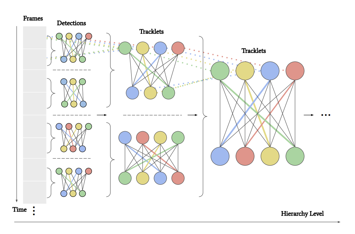
Meaning; at every level of the hierarchy, sushi considers edges spanning across longer timespans without neither increasing the edge count, nor incurring the severe label imbalance we mentioned.

Concretely, let's say we are working with 20 objects per frame:

Level 1, small graph covering 2 frames, objects = 40 objects. Number of edges = , ratio is now

Far better ratio.

As mentioned, every block, as shown in the above image, is referred to as our SUSHI block. For each graph at level l in our hierarchy, we consider embeddings and for every node and edge , with and being their respective dimension. Our node embeddings are zero-intialized, and edge embeddings are learned from a set of intial association features.

The goal of our message-passing is to propagate embedings across the graph, hereby encoding higher-order contextual information in them. To do that, SUSHI follows time-aware neural message passing framework for steps. Which then yields embeddings . At the last step of our block, our edge embeddings are fed to a binary classifier to obtain the score representing whether they represent a correct hypothesis or not, . From there, our predicted edge scores are then rounded to result in our binary decisions using a linear program. The end result is a longer-spanning set of tracklets, from the intial ones in .

The linear program can be understood as follows: The GNN outputs independent per-edge scores, but a valid trajectory needs each node to have at most one incoming and one outgoing active edge (a detection has one predecessory, one successor). These are flow-conservation constraints:

Thresholding at 0.5 could satisfy this constraint for the most part. For the few voilating nodes, they solve a small integer LP to snap predictions to the nearest feasible binary solution. Because the constraint matrix is unimodular, the LP relazation gives an exact integer optimum, so it's quick.

(the unimodular matrix deserves its own section, point being, its fast)

Features fed into each edge before the GNN runs. 4 cue types get concatenated into 1 vector, then passed through , to become the intial edge embedding .

The 4 cue types, computed between tracklets and :

1. Appearance: average the reId embedding over all detections in each tracklet, then compare. Averaging is more robust than using one detection (which could be blurry/occluded):

1. Spatial / size /time proximity : use the closest-in-time detection of each tracklet (the endpoints where they nearly meet)

1. Motion : Motion of the tracklets over time

The motion feature is the interesting part. The idea is: if ends and begins, do their trajectories meet in the middle?

Assume ends before starts. Estimate each tracklet's pixel velocity . Pick the midpoint time between them:

Then we can extrapolate both toward that midpoint, push u's last box forward, push v's first box backward.

If and are the same object, these 2 predicted boxes should land in nearly the same place. Measure that overlap with GIoU:

Notes:

• = bounding box of u's last detection; = box of v's first detection

• Meeting halfway (rather than propagatin one all the way to the other) keeps the prediction horizon short -> less drift -> more reliable.

• GIoU is used over plain IoU because GIoU still gies a meaningfull gradient/signal when the 2 boxes don't overlap at all, whereas IoU is flat at 0.

SUSHI blocks share weights, as they use the same GNN architecture. With this shared weight approach, they calculate an embedding: for each level. This embedding is then added to the output produced by , and allow the edge embeddings to encoding the feature differences that are expected at each hiarchy level. The paper mentions that this has improved not only in reducing parameter count, but also improved performance and convergence speed.

2.3 Training

The message-passing GNNs are trained jointly across all levels. For this to be possible, we unfreeze levels from first to last. There will then be iterations per level, which has the value of 500 in the paper's implementation. After all levels are unfrozen, they are then trained jointly together, this then allows them to adapt to the particular tracklet statistics produced by their predecessors.

Each level uses a focal loss over the binary edge classification scores, and sum losses over all levels to obtain the final loss.