MatIntro week 6: functions of several variables — open sets, limits, continuity and directional derivatives

Week 6 of MatIntro at KU, from Kro's Funktioner af flere variable — open and closed sets, limits that depend on the path, continuity and the extreme value theorem, directional and partial derivatives, C¹ functions. Plus solved exercises and assignment 5.

This post was AI-generated from the week's assigned reading and my course notes.

Course: MatIntro 2026, University of Copenhagen. From this week the course follows Tore August Kro, Funktioner af flere variable (TK). The reading is TK 2.1–2.4.3, pp. 41–74. Numbers like "Example 2.30" are the book's; "TKO 2.15" means exercise 2.15 in the same notes.

The chapter opens with a worry. Knowing only that is a function says nothing about its shape: and can both be while is something else entirely, and the graph can be a cloud of points. The question the chapter sets out to answer is whether there is a usable criterion for a function to behave the way intuition expects. The answer is continuity, and getting there needs a vocabulary for sets in first.

Open and closed sets (TK 2.1)

Informally (p. 42), for a set :

the boundary is the points that separate from what lies outside it — a boundary point need not belong to ;
the interior is the points of not on the boundary, completely surrounded by other points of ;
the closure is .

Formally (definition 2.9), is a boundary point of if every ball around it, however small, contains both a point of and a point outside . Then:

is open if it contains none of its boundary points — every point of is interior (definition 2.13);
is closed if it contains all its boundary points, (definition 2.14).

The book's footnote puts it well: sets are not like doors. Open and closed are not opposites, and a set can be neither or both (example 2.3). Example 2.4 runs through the cases:

Set · Boundary · Answer · the line , none of it in the set · open · the ellipse, all of it in the set · closed · · closed · , not in the set · open · empty · both open and closed · the point itself · closed

and are the only sets that are both: with an empty boundary, both conditions hold vacuously.

Bounded is a separate property (definition 2.16): fits inside some ball around the origin, for all . A rectangle is bounded; the region above a parabola, a ray, and itself are not (example 2.5).

Two more words are needed for limits. A point of is isolated if no other points of come arbitrarily close to it, and an accumulation point is a point of the closure that is not isolated (definitions 2.17–2.18). In example 2.6, has the isolated point , and its accumulation points are the closed half-plane .

TKO 2.3

Four sets built from the square with corners . The method is the book's: find the boundary, then check which boundary points belong to the set.

Exercise · Set · Boundary points in · Answer a · and · all · closed b · and · none · open c · and · the vertical sides only · neither d · · all (two full vertical lines) · closed, unbounded

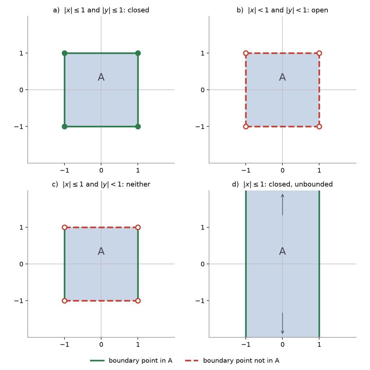The four sets of TKO 2.3; solid green boundary points belong to A, dashed red ones don't In a), the boundary is the four sides. On each side one coordinate is locked to while the other must stay within the square:

Pitfall: " and " gives only the four corners, and " or " gives four infinite lines, including points like far outside the square. Each side needs both conditions: one coordinate equal to , the other bounded by .

Pitfall: my first answer to b) was "there is no boundary". The boundary depends only on where lies, not on which points it keeps. Every ball around hits points just inside and just outside the square, so is a boundary point even though . The same square with or has the same boundary; only membership changes, and that is exactly what decides open versus closed.

In c), is in , which rules out open, and isn't, which rules out closed. On paper I wrote "both open and closed, so neither" — the right conclusion in the wrong words.

In d), there is no condition on , which means every , not . The strip is closed but unbounded, and with the open square and the open strip all four combinations of open/closed and bounded/unbounded turn up.

Limits (TK 2.2)

Distance in is the norm of the difference (definition 2.22):

With that, the definition is the one from one variable with swapped out (definition 2.23): if is an accumulation point of the domain , then means that for every there is a such that

Why an accumulation point? has to be able to approach from inside the domain. At a point outside the closure of (example 2.20) or at an isolated point (example 2.21), isn't defined anywhere nearby, and a limit means nothing.

The limit rules carry over unchanged (theorem 2.24): sums, differences, products, quotients when the denominator's limit isn't , and composition with a continuous one-variable function. When substituting works, it is all there is to it:

Example · Limit · Value 2.25 · · 2.26 · · 2.27 · · 2.28 · · , after

For forms there is no general method. Two tools from the chapter:

Polar coordinates prove that a limit exists. In example 2.29, . As , , while is, in the book's words, a malicious variable trying to spoil the calculation. But whatever does, so the expression is squeezed between and the limit is .

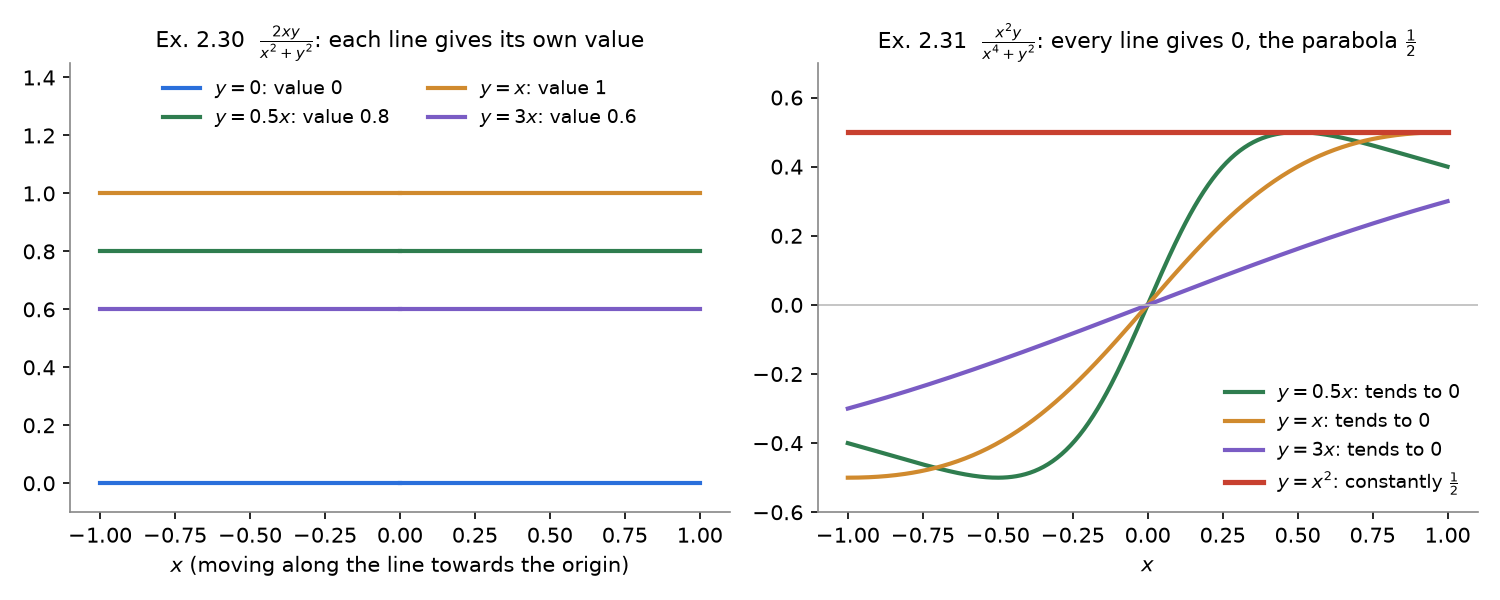
Two paths with different values prove that it doesn't. In example 2.30, is along both axes — so far it looks promising — but along it is the constant . In polar form it is : no at all, so its value depends only on the direction you come from. This is also the standard function that is continuous in and in separately without being continuous as a function of both.

Example 2.31 is the sharper warning: tends to along every straight line through the origin, and still has no limit, because along the parabola it is constantly . Checking lines is never enough to show that a limit exists.

Along each line the first function has its own constant value; the second tends to 0 along every line but is ½ along the parabola

Continuity (TK 2.3)

Definition 2.32. is continuous at if (or is an isolated point, the degenerate case). is continuous if it is continuous at every point of its domain.

In practice the definition is rarely used directly. Instead, you show the formula is built from continuous pieces:

Theorem 2.33. If and are continuous at , so are , , , and when .

Theorem 2.34. Composites of continuous functions are continuous.

So is continuous, as sums and products of constants and the coordinate functions and (example 2.36). is continuous on its domain ; outside it the function is undefined, not discontinuous (example 2.37). For a piecewise function, check that the pieces agree on the seam: in example 2.38, and both equal on .

The function from example 2.31, extended by , is the counterexample (example 2.39): continuous everywhere except at the origin, where no limit exists.

TKO 2.9a

Show that is continuous. Rename the building blocks so they don't collide with the exercise's : and . Both coordinate functions are continuous, and , so theorem 2.33 makes continuous at every point of .

The and in the theorem are placeholders, and renaming them the first time removes the confusion. Note also that is the function "take the -coordinate", not (which is here). No differentiation is involved.

The extreme value theorem (TK 2.3.1)

Theorem 2.42. If is closed and bounded, and is continuous, then has both a maximum value and a minimum value on .

This is the answer to the chapter's opening question: continuous functions on closed, bounded sets behave as intuition hopes. Both hypotheses are needed (example 2.45):

Fails · Example · What goes wrong bounded · on · grows without limit closed · on the open disc · gets arbitrarily close to , never reaches it closed · , with a boundary point not in · blows up near

The theorem says the extremes exist; it says nothing about where. In example 2.44, on the closed disc has extremes by the theorem, and they are found by another argument: increasing only shrinks , so they lie on , where has at and . The maximum is and the minimum .

Directional derivatives (TK 2.4.1)

In one variable, says a small step changes by about . In several variables the function can change differently in every direction, so the direction comes first.

Definition 2.46. For an interior point of and a vector ,

It is the ordinary derivative of along the line through in direction , measured per unit of . need not be a unit vector, so is a true slope only when ; doubling doubles the result. In example 2.47, at in direction gives and : a step of length raises by about .

The recipe:

Find the point coordinate by coordinate.
Substitute the whole point into , with brackets.
Multiply out and collect into a number plus .
Subtract : the constant cancels and every term has an .
Cancel and let .

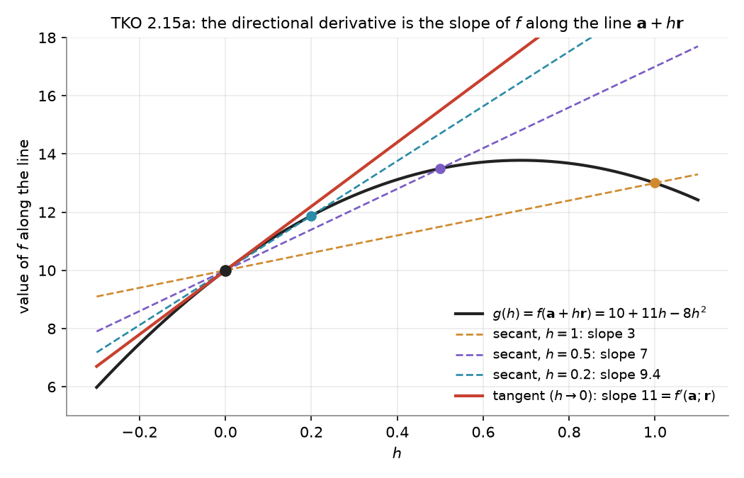
TKO 2.15a

, , .

With :

Pitfall: a number and an -term don't add up. The point went wrong twice before it was right: first , forgetting , then , adding into .

Forgetting to subtract leaves , which blows up. And is not the inside the expression; it is the value at the starting point, the same as setting .

Secants from h = 0 approach the tangent of slope 11 as h shrinks

TKO 2.15b

, , . Multiply by first, then add :

This time the is stuck inside the logarithm, so it can't be cancelled, and the quotient is of the form . L'Hôpital, with the chain rule on for and :

Pitfall: , not . The first attempt had the logarithm in the denominator and , losing the minus from .

The first guess for the point was : and added first and the sum multiplied by — the same trap as in a).

A check from lecture 6c, ahead of the reading: when is , . Here , and .

Partial derivatives (TK 2.4.2)

Definition 2.48. The -th partial derivative is the directional derivative along the -th unit vector :

Written out, only the -th coordinate moves, so in practice you differentiate with respect to and treat every other variable as a constant. For (example 2.49):

Exercises h₁–h₃

Function · ·

For with respect to , the chain rule with and gives .

Pitfall: the power rule doesn't apply when is in the exponent. My first answer was "it stays the same", which forgets the chain rule's extra factor . A check with numbers: , not .

With respect to , appears twice, so it is the product rule with and , where because is constant:

Pitfall: the first guess was ", because ". That misses two things: with respect to is , not , and the factor in front depends on too, so every term must be a product .

C¹ functions (TK 2.4.3)

Definition 2.50. A function on an open set is if its partial derivatives exist and are continuous there.

It is the criterion for "nicely differentiable" that most functions in the course pass, and it is checked the same way as continuity: compute the partials and see that they are built from continuous pieces. is (example 2.51). Only interior points matter: in example 2.52, has no partial derivative at , but those are boundary points of the domain, so the function is still on its interior.

The standard function that fails is the distance to the origin (example 2.53):

Both partials are continuous away from the origin and have no limit at it, so is on only. The graph is a cone, and its tip is a point where no tangent plane fits — the subject of part a) of this week's assignment.

Theorems used this week

Def. 2.9    a ∈ ∂A  ⟺  every ball around a meets both A and its complement
Def. 2.13   A open    ⟺  A contains none of its boundary points
Def. 2.14   A closed  ⟺  A = A ∪ ∂A
Def. 2.23   lim f(x) = L as x → a: 0 < ‖x − a‖ < δ ⟹ |f(x) − L| < ε
Thm. 2.33   f, g continuous at a ⟹ f ± g, f·g, f/g (g(a) ≠ 0) continuous at a
Thm. 2.34   composites of continuous functions are continuous
Thm. 2.42   A closed and bounded, f continuous ⟹ f has a max and a min on A
Def. 2.46   f'(a; r) = lim_{h→0} (f(a + h·r) − f(a)) / h
Def. 2.48   ∂f/∂xᵢ (a) = f'(a; eᵢ)
Def. 2.50   C¹: partial derivatives exist and are continuous on an open set

Almost everything this week is a one-variable idea with replaced by . What is genuinely new is that there are infinitely many ways to approach a point, which is why limits can depend on the path and why the derivative needs a direction.

Read next: MatIntro week 3: derivatives, the mean value theorem and L'Hôpital — The one-variable difference quotient

Assignment 5

The graded hand-in, written in LaTeX with Maple. It takes one function through five parts:

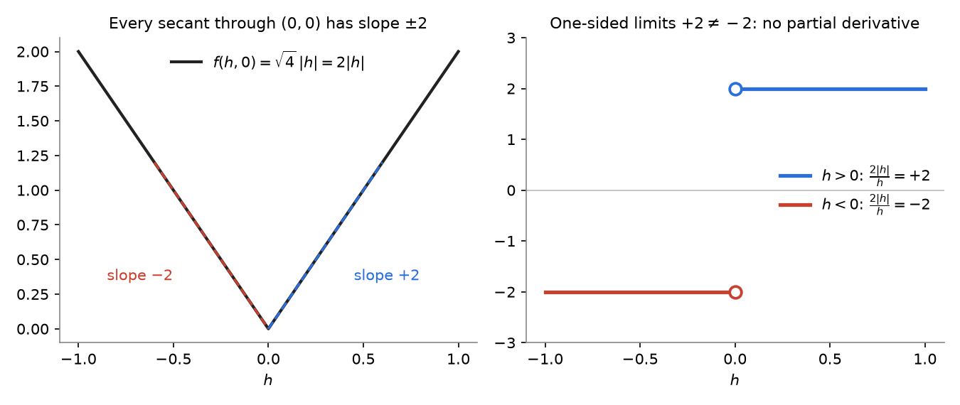
a) for , is a stretched version of the cone from example 2.53. The difference quotient at the origin is , which is from the right and from the left, so has no partial derivatives at ;
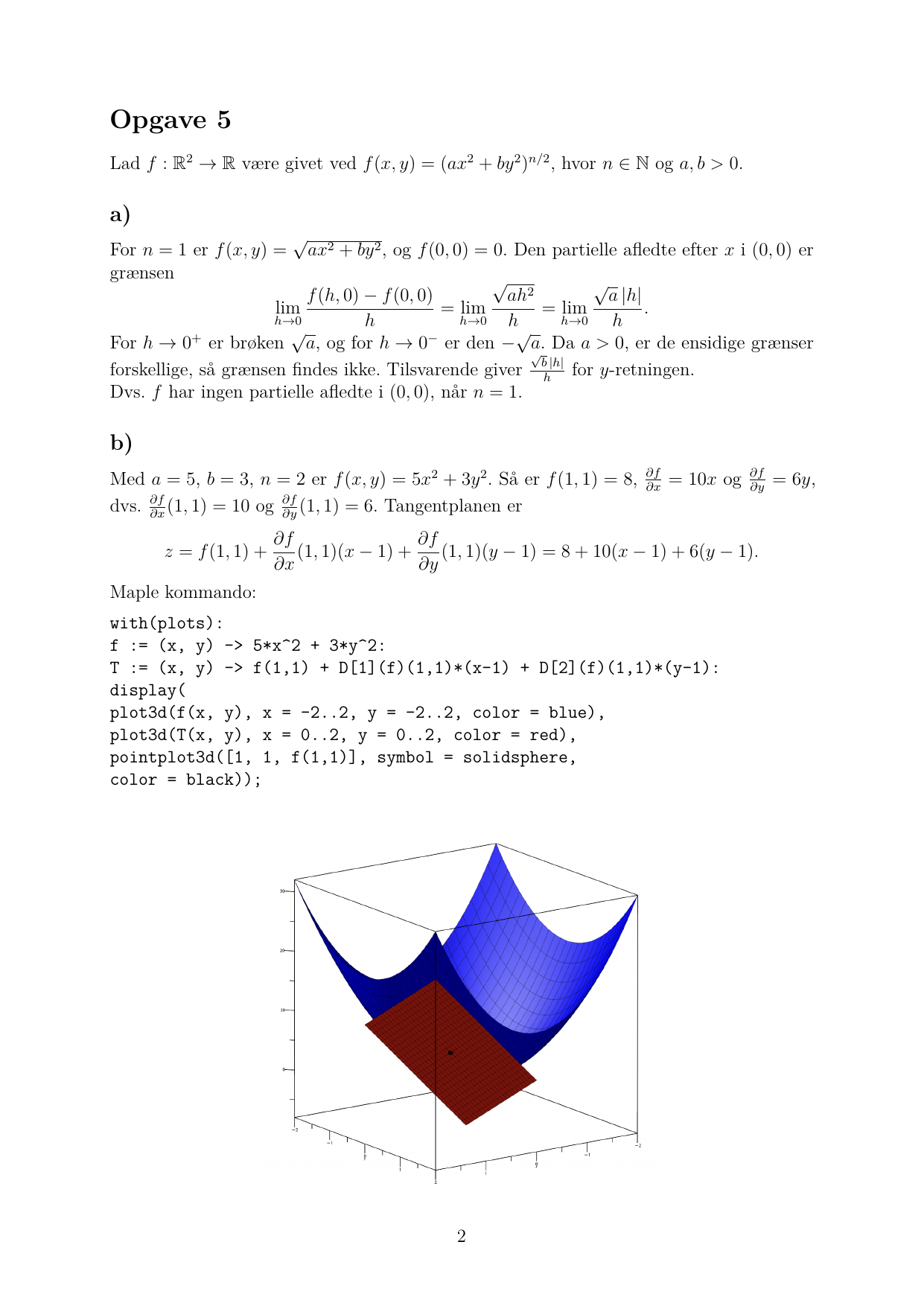
b) with , , , the tangent plane at is , plotted in Maple with the graph;
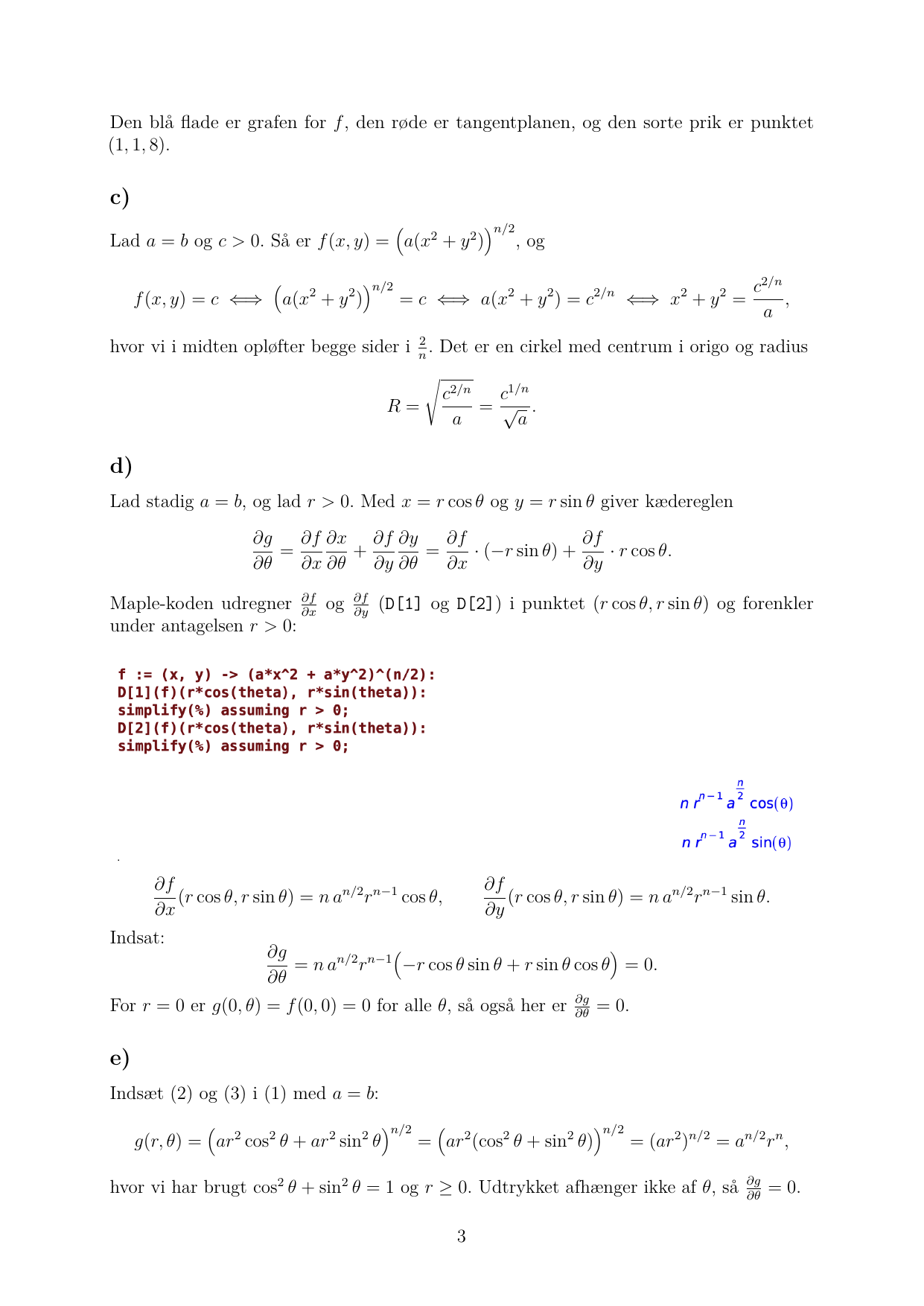
c) for the level curve is the circle with radius ;
d) in polar coordinates , and the chain rule gives ;
e) directly, , which doesn't depend on .

Parts b) to e) use tangent planes and the chain rule in several variables, which the course reaches in week 7.

Part a) with a = 4: the graph along the x-axis is a kink, and the difference quotient jumps from −2 to +2 Assignment 5, page 1 Assignment 5, page 2 Assignment 5, page 3